Risk in E+
–
Fundamental Epidemiological Concepts and Approaches
This course was developed by Dr. Kiffer G. Card, Faculty of Health Sciences, Simon Fraser University based on Dohoo, I. R., Martin, S. W., & Stryhn, H. (2012). Methods in Epidemiologic Research. VER Inc.
📚 Reference page, available throughout the lesson
This glossary collects the key concepts, people, and ideas you will meet in this lesson. Use it as a reference while you work through the material, or as a review before assessments. Type in the search box to filter entries.
⏱ Estimated reading time: 15 minutes
An earlier lesson gave us measures of disease frequency: prevalence, incidence, risk, and rate. An earlier lesson took the same probabilistic vocabulary and applied it at the level of a single test. This lesson brings these strands together: it combines the disease-frequency vocabulary with the 2×2 contingency logic to produce measures of association, the quantitative comparison between exposed and unexposed groups that is the central output of analytic epidemiology. The four content sections build up from the three ratio measures (this section: risk ratio, rate ratio, odds ratio), through difference measures and exposed-group attributable fractions (a later section), to population-level attributable measures and how each measure relates to study design (a later section), and finally to the hypothesis-testing and confidence-interval machinery that turns each of these point estimates into a defensible inference (a later section).
The section begins with the reason for measuring association, sets out the 2×2 tables from which the ratio measures are computed, defines the risk ratio, the incidence rate ratio and the odds ratio, and closes with the relationships among the three.
Measures of association assess the magnitude of the relationship between an exposure (a potential cause) and a disease. Unlike measures of statistical significance, which are heavily dependent on sample size, measures of association indicate the strength of the effect, that is, how much more (or less) likely disease is in exposed compared to non-exposed groups (Tripepi et al., 2007).
Box 6.1 sets out the difference between the strength of an association and its statistical significance, a distinction to which Section 4 returns when it introduces hypothesis tests and confidence intervals.
A measure of association tells you how strongly an exposure is linked to disease. A P-value tells you how likely the observed data would be under the null hypothesis of no association. A strong association can be non-significant (small sample), and a weak association can be highly significant (large sample). Always report both.
A measure of association compares the frequency of disease in exposed and non-exposed groups, so the data must first be arranged in a form that makes this comparison possible. The next part sets out that arrangement.
Depending on study design, disease frequency can be expressed as incidence risk, incidence rate, prevalence, or odds. The formulae later in this lesson are written in terms of the cell labels of Table 6.1, for risk data, and Table 6.2, for rate data. For risk data, the standard 2×2 table is:
Table 6.1. Layout of the 2×2 table for incidence risk data, with exposure status in the columns and disease status in the rows.
| Exposed | Non-exposed | Total | |
|---|---|---|---|
| Diseased | a1 | a0 | m1 |
| Non-diseased | b1 | b0 | m0 |
| Total | n1 | n0 | n |
For rate data, the denominator is person-time at risk rather than the number of individuals:
Table 6.2. Layout of the table for incidence rate data, giving the number of cases and the person-time at risk in each exposure group.
| Exposed | Non-exposed | Total | |
|---|---|---|---|
| Number of cases | a1 | a0 | m1 |
| Person-time at risk | t1 | t0 | t |
A quick word on odds, since the third measure below is built from them. The risk of an outcome is the number of cases divided by everyone at risk, meaning cases plus non-cases. The odds of the same outcome is the number of cases divided by the non-cases alone. If 20 of 100 people get sick, the risk is 20/100 = 0.20, but the odds are 20/80 = 0.25. Risk and odds stay close while an outcome is uncommon and pull apart as it becomes common, which is the same fact that lets the odds ratio stand in for the risk ratio only when disease is rare.
With the two layouts in place and the difference between risk and odds defined, the next part introduces the three ratio measures that are computed from these tables.
The risk ratio, the incidence rate ratio and the odds ratio each divide a measure of disease frequency in the exposed group by the same measure in the non-exposed group. Box 6.2 recalls how HSCI 230 defined the three measures and poses a short retrieval question on them.
HSCI 230 Lesson 5, Sections 1 and 2 (Introduction and Cohort Study Design; Risk-Based and Rate-Based Designs), defined the risk ratio as the risk of disease in the exposed divided by the risk in the unexposed, and the incidence rate ratio as the same comparison of incidence rates, each a count of new cases over person-time. HSCI 230 Lesson 4, Section 1 (Introduction and the Study Base), defined the odds ratio as the cross-product of the two-by-two table, the measure that a case-control study estimates. For all three, a value of 1 means no association, values above 1 mean more disease in the exposed and values below 1 mean less. This section adds which designs supply each measure and how the three relate to each other, and Section 4 adds their confidence intervals.
Retrieval question. In a cohort, 30 of 200 exposed and 10 of 200 unexposed people develop the disease. What are the risk ratio and the odds ratio?
RR = (30/200) ÷ (10/200) = 0.15 ÷ 0.05 = 3.0, and OR = (30 × 190) ÷ (10 × 170) = 5,700 ÷ 1,700 = 3.35. The odds ratio lies further from 1, as the relationships later in this section explain.
The three measures differ in the data they require, and so in the study designs that can supply them. The flip cards below give the formula for each measure and the designs from which it can be computed.
Click each card for what each measure requires of the study design:
Two worked examples show the measures in use. Worked Example 6.1 applies the risk ratio and the odds ratio to a study from Brazil that compared diarrhea among those with and without a water cistern, using the risk layout of Table 6.1.
| Water Cistern | No Cistern | Total | |
|---|---|---|---|
| Diarrhea Present | 194 | 303 | 497 |
| Diarrhea Absent | 1,588 | 1,314 | 2,902 |
| Total | 1,782 | 1,617 | 3,399 |
Both measures indicate that having a water cistern is protective against diarrhea (values < 1). The RR of 0.58 means the risk is 42% lower among those with cisterns.
Worked Example 6.2 turns to rate data in the layout of Table 6.2 and computes the incidence rate ratio for migraine in females and males aged 30 to 40.
| Female | Male | Total | |
|---|---|---|---|
| Cases of migraine | 131 | 44 | 175 |
| Person-months | 250 | 236 | 486 |
IR = (131/250) / (44/236) = 0.524 / 0.186 = 2.81
The rate of migraine is 2.81 times higher in females than males aged 30–40.
Each formula below is paired with a calculator that starts from the worked examples above. Entering the cistern data into both the risk ratio and the odds ratio calculators shows how far the two measures separate when the outcome is common.
Equation 6.1 defines the risk ratio, and Calculator 6.1 computes it, starting from the cistern data of Worked Example 6.1. Equation 6.2 defines the odds ratio, which Calculator 6.2 computes from the same data, and Equation 6.3 defines the incidence rate ratio, which Calculator 6.3 computes from the migraine data of Worked Example 6.2.
The risk ratio and the odds ratio give different values for the same data, as the cistern example shows with an RR of 0.58 and an OR of 0.53. The next part explains how the three measures are related and when one of them can stand in for another.
In general, IR values are further from the null (1) than RR values, and OR values are even further away (Cornfield, 1951; Knol et al., 2008). This can be visualised on a number line, as in Figure 6.1:
Figure 6.1. General relationships among RR, IR, and OR. OR is always furthest from the null value of 1.
Under some conditions the measures come close to one another, and the accordion below explains when the OR approximates the RR, when the RR approximates the IR, and when the OR from a case-control study estimates the IR.
When the disease is rare (prevalence or incidence risk < 5%), OR approximates RR, the classic Cornfield (1951) approximation, which showed how case-control studies such as the landmark study of smoking and lung cancer by Doll and Hill (1950) could be interpreted in terms of relative risk. This is because when a1 is small relative to n1, the denominator of the odds (b1) is approximately equal to n1, and similarly for the non-exposed group. In the cistern example, the overall risk was 14.6%, so OR (0.53) was more extreme than RR (0.58); when outcomes are not rare, treating OR as RR can substantially overstate the effect (Knol et al., 2008).
RR and IR will be close to each other if the exposure has a negligible impact on the total time at risk in the study population. This occurs when the disease is rare or when IR is close to the null value (IR ≈ 1).
OR is a good estimator of IR under certain conditions in case-control studies. If controls are selected using cumulative or risk-based sampling (all non-cases after cases have occurred), then OR estimates IR only if the disease is rare. If controls are selected using density sampling (a control selected from non-cases each time a case occurs), then OR is a direct estimate of IR regardless of disease rarity.
Interactive 6.1 shows the rare-disease condition at work: it computes the RR and the OR from one 2×2 table and plots how far the OR moves from the RR as the outcome becomes more common, so that the effect of outcome prevalence on the gap between the two measures can be seen directly.
| Y+ | Y− | Total | |
|---|---|---|---|
| E+ | 40 | 60 | 100 |
| E− | 20 | 80 | 100 |
This section has explained why association is measured, set out the layouts for risk and rate data, defined the risk ratio, the incidence rate ratio and the odds ratio, and shown that the OR lies furthest from the null and approximates the RR only when the outcome is rare. The Key Takeaways below summarise these points, the knowledge check tests them, and Section 2 turns from ratio measures to difference measures.
1. The odds ratio (OR) is the only ratio measure of association applicable to case-control studies because:
2. A risk ratio of 0.58 for diarrhea in a cistern study indicates:
3. Under what condition does OR best approximate RR?
✦ Pass the knowledge check with 100% to continue
⏱ Estimated reading time: 15 minutes
An earlier section covered the three ratio measures (RR, IR, OR), that is, how many times more likely disease is in the exposed group compared to the unexposed. This section turns to the parallel set of difference measures, which answer a different question: not how many times more, but how many extra cases occur because of the exposure. Difference measures lead naturally to attributable fractions in the exposed, which quantify how much disease in the exposed group can be attributed to the exposure itself.
The section first contrasts ratio and difference measures, then defines the risk difference and the incidence rate difference, and then turns to the attributable fraction in the exposed and its use as a measure of vaccine efficacy.
The ratio measures from an earlier section (RR, IR, OR) tell us the relative strength of association, but they do not indicate the absolute number of cases attributable to the exposure. Difference (absolute effect) measures address this gap by computing how many additional cases occur because of the exposure; the choice between ratio and difference measures is itself a substantive scientific decision rather than a statistical convenience (Greenland & Pearce, 2015; Tripepi et al., 2007).
It helps to name the two scales this contrast lives on. Ratio measures work on a multiplicative scale: a risk ratio of 2 says the exposed risk is the baseline risk multiplied by two. Difference measures work on an additive scale: a risk difference of 0.04 says the exposed risk is the baseline plus four percentage points. The same association can look striking on one scale and slight on the other, so the choice of scale is a real part of the scientific question rather than a matter of presentation.
Box 6.3 explains why both kinds of measure are needed when the public health impact of an exposure is assessed.
Even when an exposure is very strongly associated with disease (high RR), if the exposure is rare in a population, it may contribute very few cases. Conversely, a relatively weak risk factor (modest RR) that is common can be responsible for many cases. Difference measures capture this “public health impact.”
The next part defines the first of the difference measures, the risk difference, together with its counterpart for rate data, the incidence rate difference.
The risk difference (RD), also called attributable risk (Walter, 1976), is simply the risk in the exposed group minus the risk in the non-exposed group:
Similarly, the incidence rate difference (ID) is the difference between two incidence rates:
The three tabs below interpret and apply these two formulae. The first tab explains how the sign of a difference measure is read. In the second tab, Worked Example 6.3 applies Equation 6.4 to a cohort of 5,000 women followed through pregnancy, with smoking as the exposure and low birth weight as the outcome. In the third tab, Worked Example 6.4 applies Equation 6.5 to the migraine data of Worked Example 6.2. Calculator 6.4 and Calculator 6.5, which follow the tabs, reproduce the two worked examples so that the effect of changing the counts on each difference can be seen.
RD indicates the increase (or decrease) in the probability of disease in the exposed group, beyond the baseline risk. It tells you: “For every X exposed individuals, how many additional cases occur because of the exposure?”
From a cohort of 5,000 women followed through pregnancy:
| Smoker | Non-smoker | Total | |
|---|---|---|---|
| Low birth weight | 40 | 331 | 371 |
| Normal birth weight | 311 | 4,318 | 4,629 |
| Total | 351 | 4,649 | 5,000 |
For every 100 women who smoked, approximately 4.3 had a low-birth-weight baby due to the fact that they smoked (assuming causal relationship).
Using the migraine data from the previous section, 131 cases occurred among women over 250 person-months and 44 cases among men over 236 person-months.
Women aged 30 to 40 experienced about 34 more cases of migraine per 100 person-months of observation than men of the same age. The rate ratio of 2.81 from the previous section describes the same data on a relative scale.
Worked Example 6.5 takes the reciprocal of the risk difference from Worked Example 6.3 to obtain the number needed to harm, and applies the same calculation to a protective intervention to obtain the number needed to treat.
The reciprocal of a risk difference gives the number of people who must be exposed for one additional case to occur. In the smoking example, RD = 0.043, so the number needed to harm is 1 ÷ 0.043 = 23.3: about 23 women who smoke for each additional low-birth-weight baby, assuming a causal relationship.
For a protective intervention the same calculation gives the number needed to treat. If, for example, an intervention lowered the risk of an outcome from 0.20 to 0.15, RD = −0.05 and NNT = 1 ÷ 0.05 = 20 people treated for one outcome avoided.
Both numbers apply to the follow-up period of the study from which the risks come, here the pregnancy, so each is quoted with its time frame.
The risk difference and its reciprocal describe the excess risk in absolute terms. The next part expresses the same excess as a proportion of the risk in the exposed group, which gives the attributable fraction in the exposed.
The AFe (also called the attributable fraction among the exposed) expresses the proportion of disease in exposed individuals that is due to the exposure, assuming the relationship is causal (Walter, 1976). It can be viewed as the proportion of disease in the exposed group that would be avoided if the exposure were removed.
Equation 6.6 gives the AFe in three forms: from the risk difference and the risk in the exposed, from the risk ratio, and approximately from the odds ratio.
AFe ranges from 0 (where risk is equal, RR = 1) to 1 (where all disease in the exposed group is due to the exposure, RR = ∞). In case-control studies, AFe can be approximated by substituting OR for RR.
Worked Example 6.6 applies Equation 6.6 to the smoking cohort of Worked Example 6.3, and Calculator 6.6 reproduces the calculation from the two risks, from the RR or from the OR.
From the smoking example above:
Among women who smoked, 37.5% of the low-birth-weight cases were attributable to smoking. Alternatively: 0.043 / 0.114 = 0.377 ≈ 37.7% (slight rounding difference).
Vaccine efficacy is a special form of AFe, where “not vaccinated” is the exposure (factor positive) and “vaccinated” is the comparison group. Worked Example 6.7 works through a simple case, Equation 6.7 then states the general formula, and Calculator 6.7 reproduces the example. If 20% of unvaccinated individuals develop disease versus 5% of vaccinated individuals:
The vaccine has prevented 75% of the cases of disease that would have occurred in the vaccinated group if the vaccine had not been used.
Written as a formula, with Ru the risk in the unvaccinated group and Rv the risk in the vaccinated group:
Box 6.4 distinguishes the AFe, which measures the excess fraction of cases in the exposed group, from the etiologic fraction, for which the AFe provides a lower bound.
The etiologic fraction is the proportion of cases in the exposed group for which exposure was a component of the sufficient cause (Rothman, 1976). While AFe measures the excess fraction, the etiologic fraction can be higher because exposure may contribute to cases even when the baseline risk would have produced them eventually. In general, AFe provides a lower bound for the etiologic fraction (Greenland & Robins, 1988).
This section has defined the risk difference and the incidence rate difference, the numbers needed to harm and to treat, and the attributable fraction in the exposed, with vaccine efficacy as a special case. The reflection that follows asks for these measures to be computed for a single exposure, and the Key Takeaways and knowledge check consolidate the section. Section 3 moves from the exposed group to the whole population.
In a cohort study, a new environmental pollutant is found to have an RR of 3.0 for respiratory disease. The risk of respiratory disease in the non-exposed population is 2%. Calculate the risk in the exposed (RR × risk in the non-exposed), the risk difference (RD = risk in the exposed − risk in the non-exposed), and the attributable fraction in the exposed, AFe = (RR − 1) / RR. If 1,000 people are exposed, how many additional cases would you expect due to the exposure? Discuss why RD and AFe give different but complementary perspectives.
Minimum 20 characters required.
1. If the risk of disease is 12% in the exposed group and 4% in the non-exposed group, the risk difference (RD) is:
2. A vaccine efficacy of 75% means:
3. AFe = (RR − 1)/RR. If RR = 2.5, what is AFe?
✦ Pass the knowledge check with 100% and complete the reflection to continue
⏱ Estimated reading time: 12 minutes
Earlier sections worked at the level of the exposed group. This section zooms out: even if an exposure powerfully causes disease in the exposed, its public-health importance also depends on how common it is in the population. The population attributable fraction (AFp) captures this combination, and the section closes by mapping each measure of association onto the study design that produces it, tying back to earlier lessons.
The section first defines the population attributable risk and the population attributable fraction, then shows how the fraction is estimated when confounding calls for an adjusted risk ratio, and ends with a summary of the measures that each study design can supply.
While RD and AFe describe the effect of exposure among exposed individuals, public health decisions often require understanding the impact of an exposure on the entire population. Two key population-level measures address this:
The PAR is the increase in overall population risk attributable to the exposure. It reflects both the strength of the association and the frequency of the exposure in the population, an idea originally developed by Levin (1953) for lung cancer and reviewed by Northridge (1995) as a link between causal inference and public-health action.
Equation 6.8 gives the PAR in three equivalent forms, the last of which shows that it equals the risk difference multiplied by the proportion of the population that is exposed.
The population attributable fraction is the proportion of all disease in the population that is attributable to the exposure. Box 6.5 recalls how HSCI 341 Lesson 1 introduced it, and Equation 6.9 then sets out two ways of computing it.
HSCI 341 Lesson 1, Section 3 (Seeking Causes and Models of Causation), introduced the population attributable fraction with Levin's formula (1953), AFp = pe(RR − 1) ÷ [pe(RR − 1) + 1], where pe is the proportion of the population exposed. It is the proportion of disease in the whole population that is attributable to the exposure, and that would be avoided if the exposure were removed, assuming causation and no confounding. HSCI 230 Lesson 5, Section 3 (The Exposure), showed a published estimate of it for alcohol and cancer in the EPIC cohort.
Retrieval question. If 20% of a population is exposed and the risk ratio is 3, what is the population attributable fraction?
AFp = 0.20 × 2 ÷ (0.20 × 2 + 1) = 0.40 ÷ 1.40 = 0.29, so about 29% of cases would be attributable to the exposure.
This section adds a second route to the same quantity: AFp is the population attributable risk divided by the total population risk, which links it to Equation 6.8.
The second form of Equation 6.9 contains both the exposure prevalence p(E+) and the risk ratio, and Box 6.6 explains why the prevalence of exposure shapes the population impact of a risk factor.
A strong risk factor (high RR) that is rare in the population will have a small AFp. A weaker risk factor (modest RR) that is common may have a large AFp. For example, intravenous drug use has a very high RR for HIV, but if it is rare in the population, eliminating it would prevent few total cases. A modestly elevated risk factor like poor diet, affecting millions, may account for more total cases.
Worked Example 6.8 returns to the smoking and low birth weight cohort of Worked Example 6.3, computes the PAR with Equation 6.8, and divides it by the population risk, as in the first form of Equation 6.9. Calculator 6.8 and Calculator 6.9, which follow the example, reproduce the two results, and Calculator 6.9 also offers presets that compare a common, weak exposure with a rare, strong one.
From the cohort of 5,000 women (351 smokers, 4,649 non-smokers):
Only 4.1% of all low-birth-weight babies in the population were attributable to smoking. The low AFp is because very few women (351/5000 = 7%) smoked during the 2nd trimester, despite the relatively strong association (RR = 1.60).
Worked Example 6.8 used the unadjusted risks of a single cohort, and the AFp it gives assumes that the association is not confounded. The next part gives the form of the AFp that is used with a confounding-adjusted risk ratio.
If confounding is present, adjusted estimates of RR should be used. The AFp can then be estimated using:
where pd is the proportion of cases exposed to the risk factor, and aRR is the adjusted risk ratio. For multiple exposure categories, a summation formula is used.
Worked Example 6.9 applies Equation 6.10 to a hypothetical cohort study of physical inactivity and type 2 diabetes, and Calculator 6.10 reproduces the example.
Suppose a cohort study of type 2 diabetes finds that 45% of the people who developed diabetes were physically inactive at baseline (pd = 0.45), and that the risk ratio for inactivity, adjusted for age and body mass index, is aRR = 1.6 (hypothetical values).
AFp = 0.45 × (1.6 − 1) / 1.6 = 0.45 × 0.375 = 0.169, or about 17%.
About 17% of the diabetes cases in this population would be attributable to physical inactivity, assuming a causal relationship and that the adjustment has removed the confounding. The factor (aRR − 1)/aRR is the attributable fraction among the exposed, and multiplying it by the proportion of cases who were exposed scales it to the whole population.
The measures in this section and the two before it differ in the data they require. The next part sets out which of them each study design can supply.
Not all measures can be computed from all study designs. Table 6.3 summarises which measures are available:
Table 6.3. Measures of association that can be computed from cross-sectional, cohort and case-control studies.
| Measure | Cross-sectional | Cohort | Case-control |
|---|---|---|---|
| RR | ✓ | ✓ | |
| IR | ✓ | ||
| OR | ✓ | ✓ | ✓ |
| RD | ✓ | ✓ | |
| AFe | ✓ | ✓ | ✓b |
| PAR | ✓ | ✓a | |
| AFp | ✓ | ✓a | ✓c |
a Requires independent estimate of p(D+) or p(E+). b Estimated using OR. c Requires OR and independent estimate of p(E+|D+).
This section has extended the measures of Section 2 from the exposed group to the whole population, shown how a confounding-adjusted risk ratio enters the AFp, and matched each measure to the designs that can supply it. The reflection that follows applies Equation 6.9 to two risk factors that differ in strength and prevalence, and the Key Takeaways and knowledge check consolidate the section. Section 4 turns to the precision of these estimates.
Consider two risk factors for a disease: Factor A has RR = 5.0 and affects 2% of the population. Factor B has RR = 1.5 and affects 40% of the population. Calculate AFp for each factor using the formula AFp = p(E+)(RR − 1) / [p(E+)(RR − 1) + 1]. Which factor would you prioritise in a public health intervention, and why?
Minimum 20 characters required.
1. A risk factor has RR = 4.0 but affects only 1% of the population. The AFp is:
2. Which measure cannot be computed directly from a case-control study?
3. PAR differs from RD in that:
✦ Pass the knowledge check with 100% and complete the reflection to continue
⏱ Estimated reading time: 15 minutes
Earlier sections produced point estimates of association: single numbers like RR = 2.5 or AFp = 30%. Those numbers are useless without a quantification of how uncertain they are. This section closes the lesson by introducing the standard error, hypothesis tests, and confidence intervals, the same statistical-inference machinery you previewed in an earlier course, now applied directly to the measures you just learned to compute.
The section first defines the standard error of each measure, then uses it in hypothesis tests and confidence intervals, and ends with a guide to choosing a statistical test for other kinds of outcome and comparison.
The standard error (SE) provides a measure of the precision of a point estimate, that is, how much uncertainty exists in the estimate. This part gives the variance of the risk difference (Equation 6.11) and of the log risk ratio and the log odds ratio (Equation 6.12 and Equation 6.13), each with a worked example on the smoking and low birth weight cohort and a calculator. For difference measures (RD, ID), the variance can be computed directly:
Worked Example 6.10 applies Equation 6.11 to the smoking cohort, and Calculator 6.11 reproduces the calculation so that the contributions of the two groups to the variance can be compared.
For the smoking and low birth weight cohort, a1/n1 = 40/351 = 0.1140 and a0/n0 = 331/4,649 = 0.0712.
Almost all of the variance comes from the exposed group, because it contains only 351 women. The estimate would become more precise mainly through a larger exposed group.
For ratio measures (RR, IR, OR), the variance is computed on the log scale using Taylor series approximations:
The first tab gives the variance of ln(RR) (Equation 6.12), which Worked Example 6.11 applies to the smoking cohort and Calculator 6.12 reproduces. The second tab gives the variance of ln(OR) (Equation 6.13), which Worked Example 6.12 applies to the same cohort and Calculator 6.13 reproduces.
For the smoking cohort (a1 = 40, n1 = 351, a0 = 331, n0 = 4,649):
var(ln RR) = 1/40 − 1/351 + 1/331 − 1/4,649 = 0.025000 − 0.002849 + 0.003021 − 0.000215 = 0.024957, so SE(ln RR) = √0.024957 = 0.158.
The term 1/40 is by far the largest, because the exposed group has only 40 cases.
For the smoking cohort (a1 = 40, a0 = 331, b1 = 311, b0 = 4,318):
var(ln OR) = 1/40 + 1/331 + 1/311 + 1/4,318 = 0.025000 + 0.003021 + 0.003215 + 0.000232 = 0.031468, so SE(ln OR) = √0.031468 = 0.177.
The variance of ln(OR) is larger than that of ln(RR) for the same data, so the odds ratio is estimated slightly less precisely.
The standard errors computed in this part are used in the Wald statistic and in the confidence intervals later in this section. The next part turns to hypothesis testing.
A hypothesis test asks how likely the observed data would be if there were no association between exposure and disease. Box 6.7 recalls how HSCI 230 defined the p-value and separated statistical significance from practical significance, and the paragraphs that follow it state the null hypotheses for the measures in this lesson.
The glossary of HSCI 230 Lesson 11 defined the p-value as the probability, assuming the null hypothesis is true, of observing data at least as extreme as those obtained. It says nothing directly about the probability that the null hypothesis is true or about the size of an effect. HSCI 230 Lesson 12, Section 2 (Stepwise Critical Appraisal), separated statistical significance from practical, clinical or public health significance: a very large study can detect, with a small p-value, an effect too small to change any decision.
Retrieval question. A study of 200,000 people finds a risk ratio of 1.03 with p = 0.001. Is the association statistically significant, and is it practically important?
It is statistically significant at the 5% level, because p is below 0.05. A 3% relative increase is small, so its practical importance depends on how common the outcome and the exposure are; the small p-value reflects the precision of a very large study, and the risk ratio with its confidence interval carries the practical message.
For a measure of association, the null hypothesis states that there is no association:
An alternative hypothesis can be 1-tailed or 2-tailed. In general, 2-tailed hypotheses are preferred because 1-tailed hypotheses are harder to justify.
Box 6.8 describes what is lost when a P-value is reduced to a verdict of significant or non-significant.
P-values are often dichotomised into “significant” or “non-significant” at α = 0.05, but this entails a huge loss of information (Wasserstein & Lazar, 2016; Greenland et al., 2016). A P-value of 0.049 and 0.051 lead to different conclusions despite being virtually identical. Always report the actual P-value and a confidence interval, which conveys both significance and precision.
Four test statistics are in common use for measures of association: the Pearson χ², exact tests, the Wald statistic and the likelihood ratio test. The flip cards below describe each statistic and the conditions under which it applies.
Click each card to explore:
The Pearson χ² and the Wald statistic can both be calculated by hand. The tabs below give each formula with a worked example and a calculator.
The first tab gives the Pearson χ² statistic (Equation 6.14). Worked Example 6.13 applies it to the smoking and low birth weight table, and Calculator 6.14 reproduces the example. The second tab gives the Wald statistic (Equation 6.15), which Worked Example 6.14 applies to the risk difference and the risk ratio of the same cohort, using the standard errors from Worked Example 6.10 and Worked Example 6.11, and which Calculator 6.15 reproduces.
For the smoking and low birth weight table, the expected number of low-birth-weight babies among smokers, if smoking and birth weight were unrelated, is (371 × 351) / 5,000 = 26.0442, compared with 40 observed. The four expected counts are 26.0442 (a1), 344.9558 (a0), 324.9558 (b1), and 4,304.0442 (b0).
χ² = (40 − 26.0442)²/26.0442 + (331 − 344.9558)²/344.9558 + (311 − 324.9558)²/324.9558 + (4,318 − 4,304.0442)²/4,304.0442 = 7.478 + 0.565 + 0.599 + 0.045 = 8.69.
With 1 degree of freedom, χ² = 8.69 corresponds to P = 0.003, so an association this strong would be unlikely if smoking and low birth weight were unrelated.
For the risk difference in the smoking cohort, RD = 0.0428 and SE(RD) = 0.0174. Under the null hypothesis θ0 = 0, Z = (0.0428 − 0) / 0.0174 = 2.46, which corresponds to a two-sided P-value of 0.014.
For the risk ratio, the statistic is computed on the log scale with θ0 = 1: Z = (ln 1.6006 − ln 1) / 0.158 = 0.4704 / 0.158 = 2.98, with a two-sided P-value of 0.003.
Box 6.8 noted that a confidence interval conveys both significance and precision. The next part defines the confidence interval and shows how it is computed for the difference and ratio measures of this lesson.
A confidence interval (CI) reflects the level of uncertainty in a point estimate. A 95% CI means that if the study were repeated many times under identical conditions, 95% of the computed CIs would contain the true parameter value. This is a property of the procedure, not a probability statement about the parameter (Greenland et al., 2016).
The method of computing a confidence interval depends on whether the measure is a difference or a ratio. Equation 6.16 gives the interval for a difference measure and Equation 6.17 the interval for a ratio measure, and each is followed by a worked example on the smoking cohort and a calculator.
For difference measures, the CI is computed directly:
Worked Example 6.15 applies Equation 6.16 to the risk difference, and Calculator 6.16 reproduces it.
For the smoking cohort, RD = 0.0428 and var(RD) = 0.000302, so SE(RD) = √0.000302 = 0.0174.
0.0428 ± 1.96 × 0.0174 = 0.0428 ± 0.0341, giving a 95% CI from 0.0087 to 0.0769 (0.009 to 0.077 after rounding, as in Table 6.4).
The interval excludes 0. It indicates that smoking is compatible with anywhere from about 1 to 8 additional low-birth-weight babies per 100 women who smoke.
For ratio measures, the CI is computed on the log scale and then exponentiated:
The CI is symmetrical about lnθ but not about θ itself, which is why confidence intervals for ratio measures appear asymmetric.
Worked Example 6.16 applies Equation 6.17 to the risk ratio and compares the result with the interval for the odds ratio, and Calculator 6.17 reproduces both intervals.
For the smoking cohort, RR = 1.6006 and var(ln RR) = 0.024957, so SE(ln RR) = 0.15798 and the margin on the log scale is 1.96 × 0.15798 = 0.30964.
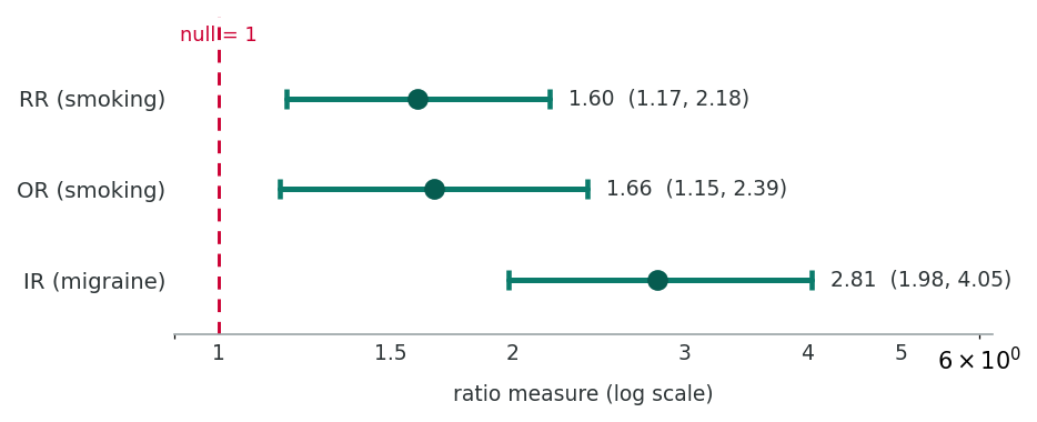
The interval runs from about 0.43 below the estimate to about 0.58 above it, the asymmetry described above. Applying the same formula to the odds ratio (OR = 1.678, var(ln OR) = 0.031468) gives 1.185 to 2.375. Table 6.4 lists 1.154 to 2.387 for the OR because the textbook computed that interval by a different method, and small differences of this kind between interval methods are expected.
A computed interval can be read in two ways: as a test of the null value and as a range of plausible effect sizes. Box 6.9 sets out both readings for ratio and difference measures, and Box 6.10 applies the first of them to the intervals for the smoking and migraine examples, which Table 6.4 lists.
However, this “surrogate significance test” is an under-use of the CI. The CI also shows the range of plausible effect sizes, which is far more informative than a binary significant/non-significant classification.
Table 6.4. Point estimates and 95% confidence intervals for the smoking and migraine examples, as reported in the textbook.
| Measure | Point Estimate | 95% CI |
|---|---|---|
| RD (smoking) | 0.043 | (0.009, 0.077) |
| RR (smoking) | 1.601 | (1.174, 2.182) |
| OR (smoking) | 1.678 | (1.154, 2.387) |
| ID (migraine) | 0.338 | (0.232, 0.443) |
| IR (migraine) | 2.811 | (1.983, 4.050) |
None of the CIs for ratio measures include 1, and none for difference measures include 0, confirming statistical significance for all associations.
The next part turns from the measures of association in this lesson to the choice of a statistical test for other kinds of outcome and comparison.
The Pearson χ², Fisher’s exact, Wald, and likelihood ratio tests above are the workhorses for 2×2 tables and the regression-based measures of association you will meet in a later course. But epidemiological analyses often require comparing means, proportions, or whole distributions across groups, sometimes paired, sometimes not, sometimes badly skewed. The right test depends on three structural questions about your data:
The matrix in Table 6.5 answers those three questions together. Find the row whose outcome type and comparison structure match your data, then read across to the test. The parametric column assumes approximate normality (or a large enough sample to appeal to the central limit theorem), and the rank-based column is the fallback when that assumption cannot be defended, when the sample is small, or when the outcome is ordinal and the spacing between its categories is not meaningful.
Table 6.5. Choosing a statistical test by outcome type, comparison structure and distributional assumptions.
| Outcome variable | Comparison | Parametric / standard test | Rank-based or exact alternative | What to report alongside the p-value |
|---|---|---|---|---|
| Continuous | One group against a hypothesised value | One-sample t-test | Wilcoxon signed-rank | Mean (or median) difference with 95% CI |
| Continuous | Two independent groups | Two-sample t-test (usually the Welch version) | Mann–Whitney U (Wilcoxon rank-sum) | Difference in means with 95% CI |
| Continuous | Two paired observations | Paired t-test | Wilcoxon signed-rank on the differences | Mean within-pair change with 95% CI |
| Continuous | Three or more independent groups | One-way ANOVA | Kruskal–Wallis | Group means, then pairwise contrasts with a multiplicity adjustment |
| Continuous | Ordered exposure categories (dose, quartile, stage) | Linear contrast within ANOVA, or regression on the category score | Jonckheere–Terpstra trend test | Change in mean per category step with 95% CI |
| Ordinal | Two independent groups | Not recommended; the numeric codes do not carry equal spacing | Mann–Whitney U | Median and IQR by group, or the proportional-odds OR from an ordinal model |
| Ordinal | Three or more independent groups | Not recommended, as above | Kruskal–Wallis | Median and IQR by group |
| Ordinal | Two paired observations | Not recommended, as above | Wilcoxon signed-rank | Median of the within-pair differences |
| Binary | Two independent groups | Pearson χ² | Fisher’s exact test when any expected count is below 5 | Risk difference, risk ratio, or odds ratio with 95% CI |
| Binary | Paired or matched | McNemar’s χ² on the discordant pairs | Exact binomial on the discordant pairs | Matched odds ratio b/c with 95% CI |
| Binary | Ordered exposure categories | Cochran–Armitage test for trend | Exact trend test | Odds ratio per category step with 95% CI |
| Nominal, 3+ categories | Any categorical exposure | Pearson χ² on the r × c table | Fisher–Freeman–Halton exact test | Cramér’s V, or category-specific odds ratios against a reference |
| Two continuous | Association between them | Pearson r (linear) | Spearman ρ (monotonic) | Coefficient with 95% CI |
| Ordinal with ordinal or continuous | Association between them | Not recommended, as above | Spearman ρ, or Kendall’s τb when ties are common | Coefficient with 95% CI |
Box 6.11 lists three judgements that remain with the analyst after Table 6.5 has been consulted.
Table 6.6 summarises the tests most commonly reported alongside measures of association.
Table 6.6. When each test is used, how it is calculated and how it is interpreted.
| Test | When to use | How calculated | How to interpret |
|---|---|---|---|
| One-sample t-test | Compare a single sample mean to a known/hypothesised value μ0; continuous, approximately normal (or n large). | t = (x̄ − μ0) / (s/√n); df = n−1. | If p < α (or 95% CI for the mean excludes μ0), the population mean differs from μ0. |
| Two-sample (independent) t-test | Compare means of 2 independent groups; continuous, approximately normal. Welch’s version does not assume equal variances. | t = (x̄1 − x̄2) / SEdiff; df = n1+n2−2 (Student) or Welch–Satterthwaite df (Welch). | p < α → the two group means differ. Always report the mean difference and its 95% CI. |
| Paired t-test | Two related observations on the same unit (before/after, twin pairs, matched cases-controls); continuous differences approximately normal. | Compute within-pair differences di; t = d̄ / (sd/√n); df = n−1. | p < α → mean within-pair change ≠ 0. Reduces between-subject variability, and is usually more powerful than treating data as unpaired. |
| One-way ANOVA | Compare means across 3+ independent groups; continuous, approximately normal, roughly equal variances. | F = MSbetween / MSwithin; df1 = k−1, df2 = N−k. | Significant F → at least one group mean differs. Follow with post-hoc pairwise comparisons (Tukey HSD, Bonferroni) to see which. |
| Pearson χ² | Test independence of two categorical variables (any r×c table). Assumption: all expected counts > 1 and ≥ 80% > 5. | χ² = Σ(O−E)²/E; df = (r−1)(c−1). Expected = (row total × column total) / N. | p < α → row and column variables are associated. The test signals whether there is association; report a measure of association (OR, RR) for strength. |
| Fisher’s exact test | 2×2 (or larger) tables with small expected counts where the χ² approximation is suspect. | Hypergeometric: enumerates every table with the same margins, sums probabilities of tables as extreme or more extreme than observed. | Exact p-value, with no large-sample assumption. With modern computing, fine to use even when χ² would also be valid. |
| McNemar’s test | Paired/matched binary outcomes (before/after on the same person; matched case-control on exposure; agreement of two diagnostic tests). | Look only at discordant pairs b and c: χ² = (b−c)² / (b+c); df = 1. Concordant pairs ignored. | p < α → the discordant pairs are unbalanced, so a real change/effect exists. The matched OR is b/c. |
| Wilcoxon signed-rank | Non-parametric alternative to one-sample / paired t-test. Use when differences are skewed, ordinal, or have outliers. | Rank |di|, attach signs, sum positive (or negative) ranks; compare to its null distribution (or large-sample z). | p < α → the median difference is non-zero (under symmetry). Robust to outliers. |
| Mann–Whitney U (Wilcoxon rank-sum) | Non-parametric alternative to two-sample t-test. Two independent groups, continuous or ordinal. | Pool all observations, rank them, sum ranks in one group; U = R1 − n1(n1+1)/2. | p < α → the two distributions differ. If shapes are similar, this is a test of medians; otherwise it tests stochastic dominance. |
| Kruskal–Wallis | Non-parametric alternative to one-way ANOVA. 3+ independent groups; continuous or ordinal. | H from rank sums; approximately χ²k−1 under H0. | p < α → at least one group’s distribution differs. Follow with pairwise rank-sum tests (Dunn’s test or pairwise Wilcoxon with adjustment). |
| Pearson correlation (r) | Linear association between two continuous variables; assumes approximate bivariate normality, sensitive to outliers. | r = Σ(x−x̄)(y−ȳ) / √[Σ(x−x̄)² Σ(y−ȳ)²]; tested via t = r√[(n−2)/(1−r²)]. | Range −1 to +1: sign = direction, magnitude = strength of linear association. Always inspect a scatterplot first. |
| Spearman ρ | Monotonic (not necessarily linear) association between two ordinal or non-normally distributed continuous variables. | Pearson r applied to the ranks of x and y. | Same −1 to +1 interpretation, but for monotonic association. Robust to outliers and non-linearity. |
Table 6.6 recommends pairwise comparisons after a significant one-way ANOVA or Kruskal–Wallis test, and Box 6.12 recalls how the significance threshold is adjusted for such multiple comparisons.
HSCI 230 Lesson 5, Section 7 (Randomised Controlled Trials: Conduct, Analysis, Vaccine Trials and Reporting), introduced the Bonferroni correction for multiple comparisons: when k comparisons are tested, each is tested at α ÷ k, so that the chance of at least one false positive across all of them stays at or below α. After a significant one-way ANOVA the comparisons are usually all pairs of groups. The Holm procedure is a less conservative alternative to Bonferroni: it orders the p-values from smallest to largest, tests them in turn against α ÷ k, α ÷ (k − 1) and so on, and stops at the first one that is not significant. Tukey's honestly significant difference is the usual method for all pairwise comparisons of means after ANOVA. A single primary outcome and comparison, named before the data are analyzed, avoids most multiplicity problems.
Retrieval question. A study makes four comparisons with an overall α of 0.05. What threshold does the Bonferroni correction set for each comparison?
0.05 ÷ 4 = 0.0125.
Box 6.13 closes the part with a rule that applies to every test in Table 6.5 and Table 6.6: each test is reported together with an effect estimate and its confidence interval.
None of the tests above are themselves measures of effect size. A statistically significant chi-square confirms that some association exists, but the magnitude must come from the OR, RR, mean difference, or correlation coefficient. Likewise, a non-significant t-test in a small study is not evidence of no effect. Always pair every test with the corresponding effect estimate and its 95% CI.
This section has defined the standard error of each measure, set out the test statistics in common use for measures of association, used the standard error in the Wald statistic and in confidence intervals, and shown how a test is chosen for other kinds of outcome and comparison. The reflection that follows compares two studies by strength of association, statistical significance and precision, and the Key Takeaways and knowledge check consolidate the section.
A study reports an OR of 1.45 with a 95% CI of (0.92, 2.28). A second study reports an OR of 1.15 with a 95% CI of (1.02, 1.30). A confidence interval that includes 1.0 indicates that the association is not statistically significant at the 5% level, and a narrower interval indicates a more precise estimate. Compare these two findings in terms of: (a) strength of association, (b) statistical significance, and (c) precision. Which finding might be more concerning from a public health perspective, and why?
Minimum 20 characters required.
1. A 95% confidence interval for an odds ratio is (1.2, 3.8). This means:
2. Why are confidence intervals for ratio measures (like OR) asymmetric around the point estimate?
3. Which test statistic is generally considered superior in regression settings?
✦ Pass the knowledge check with 100% and complete the reflection to continue
⏱ Estimated time: 20 minutes
This lesson translated the disease-frequency measures of an earlier lesson into measures of association between an exposure and an outcome. You worked through the three ratio measures (RR, IR, OR), the difference measures of effect in the exposed (RD, AFe), the population-level extensions (PAR, AFp), and the inferential machinery (standard errors, hypothesis tests, confidence intervals) that surrounds every estimate.
Lesson 7, Designing Against Bias, uses these measures to examine validity and confounding in study protocols, and Lesson 8, Time-to-Event Data, applies them to survival curves and hazard ratios. The measures you computed here will reappear in each of those lessons as the outputs that designs deliver and that systematic reviews eventually pool. For deeper treatment of these measures and their statistical foundations, see Greenland and Pearce (2015) and the historical landmark papers by Cornfield (1951) and Doll and Hill (1950).
A colleague presents findings from a case-control study showing OR = 2.3 (95% CI: 1.1, 4.8) for the association between a workplace chemical exposure and bladder cancer. She concludes the chemical “causes 2.3 times the risk of bladder cancer.” In a case-control study participants are selected on outcome status, so absolute risks and risk ratios cannot be estimated directly; the odds ratio approximates the risk ratio only under the rare disease assumption (the outcome is uncommon, roughly under 5%, in the source population); and a confidence interval that excludes 1.0 indicates statistical significance at the 5% level but says nothing about bias or confounding. Evaluate this statement. What can and cannot be concluded from this study? Discuss the roles of strength of association, statistical significance, the rare disease assumption, and the distinction between OR and RR.
Minimum 20 characters required.
Complete all 15 questions below with 100% accuracy to finish this lesson. You must also complete the reflection above before submitting.
1. Measures of association differ from measures of statistical significance in that they:
2. In a cohort study, 150 of 2,000 exposed individuals and 75 of 2,000 non-exposed individuals develop the disease. What is the risk ratio?
3. The odds ratio can be calculated from a case-control study because:
4. RD = 0.043 in the smoking and low-birth-weight example means:
5. If RR = 4.0, the attributable fraction in the exposed (AFe) is:
6. Vaccine efficacy of 80% indicates:
7. A common risk factor with a modest RR may have a larger AFp than a rare risk factor with a high RR because:
8. PAR is best described as:
9. The null value for the risk ratio (RR) is:
10. A 95% CI for RR of (0.85, 1.32) suggests:
11. Confidence intervals for OR are asymmetric around the point estimate because:
12. In the formula var(ln OR) = 1/a1 + 1/a0 + 1/b1 + 1/b0, increasing all cell counts will:
13. Which of the following measures CANNOT be estimated from a case-control study unless external data on disease incidence are available?
14. The Pearson χ² test is most appropriate when:
15. A study finds RR = 1.8 (P = 0.40). Which interpretation is most appropriate?
✦ Complete the final reflection above before submitting