Cohort
Studies
Evaluating Epidemiological Research
This lesson follows exposed and unexposed people forward in time. It covers the design, analysis, and reporting of cohort studies, and then randomised controlled trials and other experimental designs, in which the investigator assigns the exposure that a cohort study can only observe.
Learning objectives for this lesson:
- Distinguish between open and closed source populations as they relate to cohort study design
- Describe the major design features of risk-based and rate-based cohort studies
- Identify hypotheses and population types consistent with risk-based and rate-based cohort studies
- Elaborate the principles used to select and measure the exposure in cohort studies
- Design and implement a valid cohort study to investigate a specific hypothesis
- Design a randomised controlled trial that produces a valid and efficient evaluation of an intervention: state its objectives, specify the target and source populations, and describe the phases of clinical research from Phase 0 through Phase IV
- Allocate subjects using simple, stratified, cross-over, factorial, cluster, and split-plot randomisation; distinguish single, double, and triple blinding and the bias each prevents; and compute sample size requirements, including the inflation factor for cluster randomised trials
- Compare intention-to-treat and per-protocol analyses, define direct, indirect, and total vaccine efficacy, and apply the CONSORT 2025 reporting standards to plan and report a randomised trial
This course was developed by Dr. Kiffer G. Card, Faculty of Health Sciences, Simon Fraser University.
Glossary: Key Terms, People & Concepts
📚 Reference page, available throughout the lesson
This glossary collects the key concepts, people, and ideas you will meet in this lesson. Use it as a reference while you work through the material, or as a review before assessments. Type in the search box to filter entries.
Introduction & Cohort Study Design
⏱ Estimated reading time: 20 minutes
Introduction and Overview
An earlier lesson ended with a promise: cohort studies invert the case-control logic by sampling on the exposure rather than the disease, and that inversion lets us measure incidence directly without the rare-disease assumption that complicated odds-ratio interpretation. This lesson cashes that promise. Across seven content sections we walk from the basic logic of cohort design (this section), to the choice between risk-based and rate-based flavors that should now feel familiar from a later section, to the surprisingly difficult problem of measuring exposure in a longitudinal setting (a later section), to the practical questions of comparability, follow-up, outcome ascertainment, and analysis (a later section), and finally to the randomised controlled trial and other experimental designs, in which the investigator assigns the exposure (the last three sections). The unified-design discipline from an earlier lesson still applies; the lessons of an earlier lesson about pre-specified analysis plans apply with extra force, because cohort studies often run for decades and offer many opportunities for selective reporting.
Learning Objectives
- Describe the fundamental logic of the cohort study design.
- Distinguish between open and closed source populations.
- Differentiate between prospective and retrospective cohort designs.
- Recognise how cohort studies relate to controlled trials.
- Compare cohort and case-control designs, and identify Canadian record-linkage resources that support cohort studies.
What Is a Cohort Study?
The word cohort denotes a group of study subjects that has a defined characteristic in common. In epidemiological study design, that characteristic is usually exposure status. In a cohort study, we follow subjects from exposure to outcome (Grimes and Schulz, 2002).
Walk through the Framingham Heart Study from 1948 enrollment to three generations of follow-up. Next ▶ advances scenes.
A 7-scene retelling of the most famous cohort study ever launched: town enrollment (Dawber, Meadors, & Moore, 1951), baseline measurements, decades of follow-up, incidence comparisons, the birth of the term "risk factor" (Kannel et al, 1961), and the three generations still under study today (Mahmood et al, 2014).
Key Idea
A cohort study closely resembles a controlled trial, without the randomisation of exposure. We start with subjects who do not yet have the disease, classify them by exposure, follow them forward in time, and compare the frequency of the outcome between exposure groups.
Most frequently, the outcome is the occurrence of a specific disease, but cohort studies can also examine outcomes such as birth weight, body mass index, blood pressure, or quality of life. Subjects are usually individuals, but can also be groups (e.g., families).
The cohort design's modern reputation rests on a small number of landmark studies that the rest of this lesson will return to repeatedly: the Framingham Heart Study (Dawber, Meadors, & Moore, 1951), which gave epidemiology the term “risk factor” (Kannel et al, 1961); the British Doctors Study (Doll & Hill, 1954; Doll et al, 2004), which followed UK physicians for 50 years and pinned down the smoking–lung cancer link; the Whitehall II civil-servant cohort (Marmot et al, 1991), which exposed a graded socioeconomic gradient in chronic disease; the Nurses' Health Study (Colditz, Manson, & Hankinson, 1997); the multinational EPIC cohort (Riboli et al, 2002); and the recent generation of population biobanks, UK Biobank (Sudlow et al, 2015) and the Canadian Longitudinal Study on Aging (Raina et al, 2019).
Figure, The logic of cohort design: classify disease-free subjects by exposure, follow them forward, compare the disease frequency between groups.
Cohort and Case-Control Designs Compared
An earlier lesson built the case-control design, which starts from disease status and looks back to exposure. The table below sets the two designs side by side; read it as a guide to which direction of inquiry suits a given question.
| Feature | Cohort Study | Case-Control Study |
|---|---|---|
| Direction of inquiry | Exposure → Outcome | Outcome → Exposure |
| Starting point | Defined by exposure status | Defined by disease status |
| Measures incidence directly? | Yes | No |
| Primary measure of association | Risk ratio, rate ratio | Odds ratio |
| Best suited for | Rare exposures, multiple outcomes | Rare diseases, multiple exposures |
| Temporal sequence | Clearly established | Relies on retrospective data |
| Cost and time | Often expensive and lengthy | Generally less expensive and faster |
| Key biases | Loss to follow-up, selective attrition | Recall bias, selection bias in controls |
Why Cohort Studies Are Well Suited to Causal Questions
The ability to measure incidence directly is the central strength of the cohort design. It establishes temporal sequence (exposure precedes outcome), allows calculation of multiple measures of association, and can study multiple outcomes associated with a single exposure. For rare exposures, cohort studies are particularly efficient because you can intentionally over-sample exposed individuals.
Choosing the Right Design: A Practical Example
Suppose you want to study whether exposure to a specific industrial solvent increases the risk of a rare liver cancer. A prospective cohort study would require following thousands of exposed and unexposed workers for decades, which is extremely expensive and slow. A case-control study, by contrast, could identify 200 liver cancer cases from a cancer registry, select 400 matched controls, and assess past occupational exposure through interviews and employment records, producing results in months rather than years.
For rare diseases, case-control studies are usually the design of choice because they can efficiently identify enough cases to detect meaningful associations.
Selecting the Study Sample (Participants)
How we select the cohort depends on what we know in advance. The three flip cards below name the standard choices, click each one and notice that the choice flows from the data already in hand, not from any abstract preference for one design over another.
In both two-cohort and single-cohort designs, after selecting subjects we (1) verify they meet inclusion criteria, (2) confirm exposure status, (3) ensure they do not yet have the outcome, then (4) follow them for a defined period and compare incidence between exposure groups.
Whichever cohort structure you pick, the next decision is whether the follow-up has already happened or whether you will be doing it as the study runs.
Prospective vs. Retrospective Designs
Cohort studies can be conducted either way, depending on whether suitable records already exist (Euser et al, 2009). The two tabs below put the trade-offs side by side.
In a prospective cohort study, the disease has not yet occurred when the study begins. Subjects are recruited, exposure is assessed at baseline, and they are followed forward in time as outcomes develop.
Advantages: Allows more detailed information-gathering and careful recording of exposure, confounders, and outcome timing (see Examples 8.6, 8.7, and 8.9).
Disadvantages: Time-consuming and expensive; vulnerable to losses to follow-up over long study periods.
In a retrospective cohort study, the follow-up period has already ended and the disease event has already occurred when subjects are selected (Hudson et al, 2005). Investigators reconstruct exposure and outcome from existing records.
Advantages: Faster and cheaper; useful when good historical records exist (Examples 8.1, 8.4, 8.5).
Disadvantages: Requires suitable existing databases; depth of information is limited to what was recorded.
Beyond the timing question is a structural one about the population itself: does its membership stay fixed for the duration of follow-up, or do people enter and leave? You met this distinction in an earlier lesson; it returns here as a more central concern, because cohort follow-up is what makes it operational.
Open vs. Closed Source Populations
The nature of the source population determines the appropriate design. This is a critical decision that affects everything from sample-size calculations to the choice of analytic methods. Read the table below as a checklist for matching disease type to design type, chronic outcomes almost always require open-population, rate-based handling, and a later section builds out exactly what that requires.
| Feature | Closed Population | Open Population |
|---|---|---|
| Membership | Fixed at start of study | Subjects can enter and leave |
| Follow-up | All subjects observed for full risk period | Variable time-at-risk per subject |
| Best disease type | Short risk period (e.g., outbreaks) | Long or chronic risk period (e.g., cancers) |
| Disease frequency | Risk (cumulative incidence) | Rate (incidence density) |
| Acceptable losses | Few or none preferred (<10%) | Time-at-risk accounted for explicitly |
Key Examples
Three published examples bring the design choices we have just enumerated into one place. We will refer back to these throughout the lesson by number, so it is worth pausing on each one to identify which boxes the investigators ticked: prospective vs. retrospective, two-cohort vs. single, open vs. closed, risk-based vs. rate-based.
Choi et al (2011) conducted a hospital-based cohort study where the exposure was discharge against medical advice (DAMA) versus discharged with medical advice (DWMA). The outcome was readmission within 14 days. Each DAMA patient was matched with one DWMA patient by 10-year age group, gender, and clinical characteristics. Because all patients were observable for the full 14-day risk period, this is a classic risk-based design. Conditional logistic regression accounted for the matching. Result: 26% of DAMA patients were readmitted within 14 days versus only 3% of DWMA patients.
Crane et al (2011) conducted a retrospective cohort study based on interviews with 11,000+ women who gave birth in two Canadian provinces (2001–2009). Eleven per cent self-declared exposure to environmental tobacco smoke. Outcomes included infant body dimensions, Apgar scores, respiratory distress syndrome, and stillbirth. Multiple regression was used to control for confounders. Tobacco smoke was associated with lower birth weight, smaller body size, and increased stillbirths. Note: when outcomes are on a continuous scale (e.g., birth weight), the cohort design still applies; we just use linear rather than logistic regression.
Mehta et al (2010) used a population-based retrospective cohort to investigate falls and fractures in adults ≥50 years. The exposure was atypical versus typical antipsychotic agents. More than 60 covariates were combined into a propensity score, and the “Greedy 5-1 matching technique” was used to match subjects with similar scores. Each exposure group contained 5,580 people. While the hazard ratio did not differ significantly between drug classes, taking any antipsychotic for >90 days was associated with HR = 1.8 for falls or fractures.
The propensity score, the probability of exposure given the measured covariates, was introduced in Lesson 3, Section 1, as part of Rubin's design-before-data step.
Record-Linkage Infrastructure for Canadian Cohort Studies
The retrospective and virtual cohorts described above depend on records that someone else has already collected. Most epidemiological work in Canada does not involve enrolling a fresh cohort. Instead, researchers reuse data that have already been collected through health-system encounters, surveys, environmental monitoring, and registries. Three pieces of national infrastructure show up repeatedly:
Population Data BC (PopData BC)
A platform that links de-identified individual-level administrative data across the BC Ministry of Health, Vital Statistics, PharmaNet (every dispensed prescription), the BC Cancer Registry, MSP physician billings, hospital discharges (DAD), and education and social-services data. Researchers obtain a study-specific extract under a data access agreement.
Designs supported: retrospective cohorts such as those in this lesson; nested case-control and case-crossover designs (see the earlier lesson Case-Control Studies); ecological and spatial analyses (see the later lesson Ecological and Group-Level Studies); and intervention evaluations using natural experiments. Other provinces have analogous systems: ICES (Ontario), MCHP (Manitoba), HDNS (Nova Scotia), IRSPUM (Quebec).
Health Data Research Network Canada (HDRN Canada / SPOR DSP)
A federation of provincial data centres (PopData BC, ICES, MCHP, etc.) that supports multi-jurisdictional studies under a single application. Each centre runs the analysis behind its own firewall and only summary results are shared, so individual-level data never crosses provincial lines. Useful when you need national power or generalisability across health systems.
CANUE: Canadian Urban Environmental Health Research Consortium
A national repository of standardised, postal-code- and DA-level environmental exposures: air pollution (NO2, PM2.5, O3), greenness (NDVI), walkability, noise, climate, neighbourhood SES indices. CANUE indicators can be linked to any cohort with postal codes (including PopData BC extracts and CCHS shared files), turning subject-level health data into ecological or multilevel exposure–outcome studies.
Worked Example: A PopData BC + CANUE Cohort Study
To estimate the effect of long-term PM2.5 exposure on incident cardiovascular disease in BC adults, a researcher could:
- Define the cohort using the PopData BC Consolidation File, that is, everyone with active MSP coverage on 1 Jan 2010 (a near-complete census of BC residents).
- Pull baseline covariates from MSP and DAD (chronic conditions, comorbidity scores).
- Link each person's six-character postal code to CANUE annual PM2.5 estimates to assign exposure.
- Follow forward in DAD/Vital Stats to ascertain incident MI, stroke, and CV death (the outcomes).
- Apply Cox regression with a time-varying exposure, adjusting for area-level deprivation (also from CANUE).
This is a retrospective cohort with an environmental exposure, sitting at the boundary of cohort and ecological designs. The data come from three different stewards but no new participant was ever recruited.
Stating the Study Objective
Each study should clearly specify:
- The target population (to which inferences will be made)
- The source population (from which the study sample, the participants, will be drawn)
- The unit of observation (individuals or groups)
- The exposure, the disease, and the follow-up period
- The setting (context or venue) of interest
- If biology is known: the amount or duration of exposure thought to cause disease, and the relevant time window for exposure (current vs. lifetime vs. historical)
Key Takeaways
- Cohort studies follow disease-free subjects from exposure forward to outcome.
- The design parallels a controlled trial, minus randomisation.
- Two-cohort designs select by exposure status; longitudinal designs select a single group with a range of exposures.
- Studies can be prospective or retrospective; the difference is timing relative to outcome occurrence.
- Closed populations call for risk-based designs; open populations call for rate-based designs.
- Compared with case-control studies, cohort studies measure incidence directly and suit rare exposures and multiple outcomes; linked administrative data, such as PopData BC records joined to CANUE exposures, make large retrospective cohorts possible without recruiting anyone new.
The takeaways above name what changed conceptually compared with case-control designs. The worked example that follows makes the change concrete: because we sampled on exposure, the same kind of 2×2 table you met in earlier lessons now yields a risk ratio and an incidence rate ratio directly, no rare-disease assumption required.
Worked example: risk ratio and incidence rate ratio from cohort data
A hypothetical cohort enrols 1,000 exposed and 1,000 unexposed people who are free of the outcome and follows them for up to five years. Some participants develop the outcome or leave the study early, so the two groups contribute different amounts of person-time.
| Group | People | New cases | Person-years | Risk (cases / people) | Rate per 1,000 person-years |
|---|---|---|---|---|---|
| Exposed | 1,000 | 80 | 4,500 | 0.080 | 17.78 |
| Unexposed | 1,000 | 30 | 4,900 | 0.030 | 6.12 |
The risk ratio is 0.080 / 0.030 = 2.67, so over five years exposed people had 2.67 times the cumulative risk of the outcome. The incidence rate ratio is 17.78 / 6.12 = 2.90. It is slightly larger than the risk ratio because the exposed group contributed less person-time (4,500 against 4,900 person-years), through earlier events or earlier loss to follow-up, and a smaller denominator raises the rate.
The risk ratio answers how many times more likely an exposed person is to develop the outcome over the follow-up window. The rate ratio answers how much more frequent the outcome is per unit of person-time. In an open cohort with variable follow-up, the rate-based answer is usually the appropriate one. Both measures come directly from the cohort because it was sampled on exposure; a case-control design could only approximate them through the odds ratio.
The reflection below asks you to use the timing distinction in a concrete research scenario. After working through it and the knowledge check, a later section returns to the risk-vs.-rate split that the worked example just previewed and shows what each design buys, costs, and assumes.
Reflection
Reflection
Think of a health question you find compelling. Would you address it with a prospective or retrospective cohort design? What records or recruitment infrastructure would you need? What might be lost or gained by each choice in your specific case?
Minimum 20 characters required.
1. The fundamental logic of a cohort study is to:
2. A cohort study most closely resembles which of the following designs?
3. In a retrospective cohort study, when has the outcome event occurred relative to the start of the study?
4. Which of the following best describes a closed source population?
Risk-Based & Rate-Based Designs
⏱ Estimated reading time: 15 minutes
Introduction and Overview
An earlier section established what a cohort study is and named the design choices its investigators have to make. This section drills into the most consequential of those choices: whether to count events per person (risk) or events per unit of person-time (rate). The two designs share a 2×2 layout but differ in what they assume about the population and what they let you say about disease frequency. Sample-size planning, surprisingly, is a useful place to start, because the calculation is the same for both designs even when the analysis ends up being different.
Learning Objectives
- Describe the design and assumptions of risk-based (cumulative incidence) cohort studies.
- Describe the design and analysis of rate-based (incidence density) cohort studies.
- Identify hypotheses and population types appropriate for each design.
- Calculate and interpret the basic measures of disease frequency for each design.
Sample Size
Initial sample-size estimates are usually performed assuming an equal number of exposed and non-exposed subjects, and assuming the disease is measured by risk (Section 8.2.2). This approach is often sufficient for initial planning even if the population is open and a rate-based design must ultimately be used.
Modern Sample-Size Software
Recent software allows for unequal sample sizes, repeated measures, multivariable regression models, and proportional hazards models. Specialised methods exist for competing risks (Latouche and Porcher, 2007), survival-time outcomes (Matsui, 2005), strata-matched designs (Mazumdar et al, 2006), and time-varying exposures (Basagana et al, 2011).
Risk-Based (Cumulative Incidence) Designs
This is the simplest form of cohort study, but several assumptions must hold:
- Exposure groups are defined at the start of the study and remain unchanged (fixed cohorts).
- The study groups are closed, all subjects must be observed for the full risk period.
- There should be few or no losses (some authors use >10% losses as a cut-point that casts doubt on validity).
When Risk-Based Designs Work Best
Risk-based designs work best for diseases with a relatively short risk period (e.g., acute infections, post-surgical complications). For chronic diseases such as many cancers, where the risk period is lifelong and often longer than feasible follow-up, a rate-based design is preferred.
2×2 Table: Risk-Based Cohort Design
| Exposed | Non-exposed | Total | |
|---|---|---|---|
| Diseased | a1 | a0 | m1 |
| Non-diseased | b1 | b0 | m0 |
| Total | n1 | n0 | n |
We select n1 exposed and n0 non-exposed individuals (free of disease) from the source population, follow them for the full follow-up period, and observe a1 exposed cases and a0 non-exposed cases. The two risks of interest are:
The Denominator
In risk-based designs, the denominator is the number of subjects in each exposure category. This is only valid because every subject is observed for the full risk period, otherwise, who you count and who you don’t would depend on follow-up time.
HSCI 341 Lesson 4, Section 2 (Incidence: Risk and Rate) develops incidence risk with formula calculators, worked examples and the assumption of a closed population.
The two risks can be compared on two scales. The risk ratio divides one risk by the other; the risk difference (also called the attributable risk) subtracts them, giving the absolute difference in incidence between the exposed and unexposed groups:
In the hypothetical cohort from the worked example in an earlier section, RD = 0.080 − 0.030 = 0.050, or 50 extra cases per 1,000 exposed people over five years, alongside a risk ratio of 2.67. The absolute figure is the one that tells a health planner how many cases the exposure adds.
Risk-based designs are conceptually clean but operationally fragile, their assumptions break the moment people leave the cohort or the risk period extends beyond a few months. The rate-based alternative was developed precisely to handle the populations where those assumptions do not hold.
Rate-Based (Incidence Density) Designs
In many cohort studies, not every subject is under observation for the full risk period, especially when:
- The source population is dynamic (subjects enter and leave).
- The follow-up period is long.
- Subjects are added part-way through the biological risk period.
- A significant proportion of subjects withdraw from the study.
- Exposure status itself changes during the study.
In these situations, we cannot just count exposed and non-exposed subjects. Instead, we accumulate the amount of ‘at-risk time’ contributed by each subject in each exposure category. The denominator becomes person-time, not persons. For example, 10 people each followed for 2 years and 20 people each followed for 1 year both contribute 20 person-years, so this denominator credits every subject for exactly as long as we actually observed them.
2×2 Table: Rate-Based Cohort Design
| Exposed | Non-exposed | Total | |
|---|---|---|---|
| Diseased | a1 | a0 | m1 |
| Person-time at risk | t1 | t0 | T |
Each subject contributes ‘at-risk’ time until they develop the disease, are lost to follow-up, or the study ends. The two rates of interest are:
Choice of Analysis
If follow-up is relatively short and rates are reasonably constant, Poisson models are appropriate. If follow-up is long and the assumption of a constant rate is not tenable, survival analysis (e.g., Cox proportional hazards) is preferred (Cox, 1972; see Chapter 19).
You have now seen both designs from the inside. The next subsection puts them side by side; read it as a decision aid for matching design to research situation, not as a statement that one design is generally better than the other.
Comparing the Two Designs
Risk-based designs are best when:
- The population is closed (fixed cohort).
- The risk period is short (so all subjects can be observed for the full period).
- Losses to follow-up are minimal (under ~10%).
- Examples: acute outbreaks, surgical complications within 30 days, hospital readmissions within 14 days (Example 8.1).
Rate-based designs are best when:
- The population is open (dynamic).
- Follow-up is long or the risk period is chronic.
- Subjects enter or leave the study at different times.
- Exposure status may change during follow-up.
- Examples: rugby injury rates over a season (Example 8.6), invasive breast cancer over 10+ years (Example 8.7), fracture incidence over decades (Example 8.8).
Risk denominator: the number of subjects in each exposure category. Counts people.
Rate denominator: the cumulative person-time at risk in each exposure category. Counts time.
This means risk is dimensionless (a proportion between 0 and 1), while a rate has units of cases per person-time (e.g., 4.0 per 1,000 person-years).
HSCI 341 Lesson 4, Section 2 develops exact and approximate person-time and the conversion between risk and rate.
Key Examples
The four examples below illustrate the design choice with real published studies. The first two are risk-based; the last two are rate-based. As you expand each, ask yourself why the investigators chose what they chose, in every case the source population's behaviour and the follow-up window's length will be doing most of the work.
Kelz et al (2009) compared morbidity and mortality following 56,000+ general and vascular surgical procedures (2001–2004). Time of operation was grouped into seven 2-hour periods. Risk of mortality within 30 days had a moderately strong association with start times after 9:30 pm (OR = 1.22), and morbidity had OR = 1.32 for late-night surgeries. However, when emergency cases were excluded, no odds ratios were significant. The excess crude risk was largely explained by the nature of the clinical cases, an important reminder about confounding by indication.
Leece et al (2010) followed approximately 250 HIV-positive women receiving care at the Ottawa Hospital General Campus Immunodeficiency Clinic (2002–2005). The outcome was undergoing cervical screening; predictors included demographics, HIV status, and primary care provider status. Analysis combined χ2 tests with logistic regression. The 12 women without a primary-care provider were less likely to undergo screening (RR = 1.6) than the 84 women with providers. The authors noted that abnormal screening results were common and that recent low CD4 cell count was the only significant predictor.
Chalmers et al (2011) followed 704 male amateur rugby players (aged 13+) over a season. The ‘time’ component was a game, with a total of 6,263 player-games of follow-up. Exposures included age, ethnicity, experience, BMI, smoking, previous injury, training, weather, ground conditions, foul play, and protective equipment. Because rates were reasonably constant over the period, Poisson regression was appropriate. Notable findings: Pacific Island vs. Maori ethnicity (IR = 1.5), ≥40 hours of strenuous activity weekly (IR = 1.5), playing while injured (IR = 1.5), foul play (IR = 1.9), and headgear use (IR = 1.2).
Luo et al (2011) drew on the Women’s Health Initiative Observational Study: 90,000+ women aged 50–79 followed across 40 US clinical centres. Smoking exposure was characterised in detail (status, age started, age quit, cigarettes/day, pack-years). Over an average of 10.3 years of follow-up, 3,520 incident invasive breast cancers were identified. Because of the long follow-up, Cox proportional hazards models (rather than Poisson) were used. Findings: HR = 1.09 for former smokers and HR = 1.16 for current smokers. Among lifetime non-smokers, only those with the highest passive-smoke exposure had increased risk; no significant dose-response trend was seen.
Key Takeaways
- Risk-based designs use number of subjects as the denominator and require a closed cohort followed for the full risk period.
- Rate-based designs use person-time as the denominator and accommodate dynamic populations and variable follow-up.
- The choice between Poisson and Cox proportional hazards depends on whether the rate is reasonably constant or changes substantially over follow-up.
- Initial sample-size calculations can be done assuming a risk-based design even when the analysis will ultimately be rate-based.
The reflection below asks you to apply the choice from this section to a specific long-running occupational cohort. After working through it, a later section turns to a problem that stays mostly hidden in textbook treatments: how do you actually measure exposure when it can change over years or decades of follow-up?
Reflection
Reflection
Suppose you are studying the effect of a workplace exposure (e.g., shift work) on cardiovascular disease over 20 years. Workers can join or leave the company at any time. Which design (risk-based or rate-based) is more appropriate, and why? What practical issues would arise that wouldn’t arise in a 14-day hospital readmission study?
Minimum 20 characters required.
1. Which of the following is a key requirement of a risk-based cohort study?
2. In a rate-based cohort study, the denominator of the rate is:
3. Which study design is most appropriate when the source population is dynamic and follow-up is long?
4. When follow-up is long and the assumption of a constant rate is not tenable, which analysis is preferred?
The Exposure
⏱ Estimated reading time: 15 minutes
Introduction and Overview
Earlier sections set up the architecture of the cohort study and the choice of risk-vs.-rate design. Both treated “exposed” as if it were a fixed property of each subject. In real cohorts that is rarely true. People start smoking, quit, switch jobs, change diets; doses accumulate. This section is about how exposure is actually measured and handled when it can vary across years or decades of follow-up, the technical problem that distinguishes a working cohort study from a textbook one.
Learning Objectives
- Elaborate the principles used to select and measure exposure in cohort studies.
- Distinguish between permanent and non-permanent exposures.
- Describe the concept of an induction period and its role in time-at-risk calculations.
- Identify how dichotomous, ordinal, and continuous exposure scales differ in measurement and analysis.
Why Exposure Measurement Matters
In cohort studies, the objective is to identify the consequences of a specific exposure factor. Exposures can range from study-subject characteristics (sex, age) to infectious or noxious agents, environmental exposures, or food-related factors. Exposures that can be manipulated are of special interest because they lead more directly to disease control.
Measurement Is Not Trivial
Although measuring exposure might seem simple at first glance, careful thought should be given to how it is measured and expressed. Each study should specify what constitutes exposure and, when possible, the ‘induction period’, how long after exposure is reached before disease might reasonably arise. The more complex the exposure, the more important it is to validate the assessment.
Scales of Exposure Measurement
Exposure status can be measured on different scales, each with implications for design and analysis. The four flip cards below run from the simplest binary contrast up to compound measures that combine intensity and duration. The pattern to take away: more granular measurement makes the design better suited to detecting dose-response, but only if the underlying biology really has a graded effect.
The choice of measurement scale is independent of a second question: does the exposure stay fixed for the rest of the subject's life, or can it change?
Permanent vs. Non-Permanent Exposures
Permanent exposures are time-invariant, factors such as sex, race, or one-time exposures such as a vaccination. These are relatively easy to measure, but a moment’s thought reveals subtleties:
- Age at exposure may matter (e.g., age at vaccination, age at smoking initiation).
- Even ‘one-time’ exposures may have a threshold or dosage requirement to count as ‘exposed’.
- If the disease event occurs before exposure is completed, it should not be counted as an outcome event, the exposure could not have caused it.
In early studies, the goal may be to determine the threshold at which exposure becomes biologically meaningful (Rohan et al, 2007).
Non-permanent exposures change over time: food intake, lifestyle factors, environmental exposures, or any exposure where the timing matters. These add complexity:
- When did exposure start? (e.g., age started smoking)
- When did exposure stop? (e.g., age quit smoking)
- How intense was exposure? (cigarettes per day)
- How long did it last? (years smoked)
Sometimes a simple summary will suffice (e.g., years smoked); sometimes a compound measure (e.g., pack-years) is needed. The more information collected, the more credibly causal relationships can be inferred and the more useful the findings are for prevention.
Both permanent and non-permanent exposures share a complication that becomes visible only when you start counting person-time: the gap between when exposure happens and when disease can plausibly result.
The Induction Period & Time-at-Risk
An important concept in cohort design is the induction period, the time after exposure is completed before disease can reasonably arise.
Figure 8.1, Life experience: exposure, induction period, and time-at-risk.
Handling the Induction Period
If there is a known induction period following completion of exposure, then until that period is over, the time-at-risk of ‘exposed’ individuals should be added to the non-exposed group. Some researchers prefer to discard disease experience during the induction period because of uncertainty about its duration; this is often the safest choice provided sufficient time-at-risk remains in the exposed group to maintain precision.
Changing Exposure Status
If exposure status changes during follow-up, an individual subject can contribute time-at-risk to both exposed and non-exposed categories:
- Previously non-exposed subjects contribute to the exposed category after the exposure threshold is reached.
- Previously exposed subjects contribute to the non-exposed category after any lag effects have ended.
- If a subject develops the disease, the exposure category assigned is the one they were in at the time the outcome occurred.
Losses to Follow-Up
For subjects lost to follow-up, time-at-risk accumulates until the last date their exposure status is known. If the precise time of loss is unknown, the midpoint of the last known exposure period is conventionally used.
One last twist on the meaning of “exposure” is worth flagging before we move on, because it shows up surprisingly often in chronic-disease cohorts.
Disease as Exposure
Disease itself can serve as an exposure for other outcomes such as additional diseases, mortality, or quality-of-life measures. Lazo et al (2011) followed 11,000+ adults for 18 years using non-alcoholic fatty-liver disease (NAFLD) as the exposure. Those with NAFLD (whether or not they had elevated liver enzymes) had a similar mortality hazard ratio as those without NAFLD, an interesting null result.
Key Examples
The three published cohorts below illustrate the full range of exposure handling we just covered: a continuous diet exposure validated against multiple recalls, a multi-exposure design with biospecimens, and a multinational study that pushes from estimated relative risk to population-attributable fraction. Expand each one and notice which exposure-measurement decisions shape the rest of the design.
Warensjo et al (2011) studied women in the Swedish Mammography Cohort. Calcium intake from diet, supplements (1 dose = 500 mg), and multivitamins (1 dose = 120 mg) was the major exposure. Total calcium intake correlated well (r = 0.77) between food-frequency questionnaire and 14 repeated 24-hour recalls, an example of careful exposure validation. Cumulative dietary calcium intake (in quintiles) was related to fracture and osteoporosis incidence using Cox proportional hazards and logistic models. Findings: a chronic, low-dietary calcium intake was associated with increased fracture and osteoporosis. Above the base level, only minor differences were observed; in the highest-intake group, hip fracture rate was somewhat increased.
Rohan et al (2007) recruited alumni from three Ontario universities (1995–1998). The major outcome was new cancer incidence. Participants completed lifestyle and food-frequency questionnaires, measured waist and hip circumferences, and provided hair and toenail specimens (for trace element and DNA analysis). Of the 73,000+ recruits, 97% provided biological specimens. Exposures included exercise, lifestyle factors, molecular markers, and dietary characteristics. The paper includes a particularly good discussion of creating compound nutritional variables from food-frequency data and verifying them.
Schutze et al (2011) reported on the European Prospective Investigation into Cancer and Nutrition (EPIC; Riboli et al, 2002), a multicentre prospective cohort that recruited 520,000 men and women aged 35–70 from 10 European countries (1992–2000). Alcohol consumption was measured at recruitment in grams/day and classified as never, former, or lifetime consumer. Cancer incidence was identified through cancer registries (follow-up ended 2002–2005). The analysis combined regression coefficients with population prevalence of consumption above recommended levels. If causality is assumed, alcohol consumption beyond recommended levels was responsible for an estimated 10% of all cancers in men and 3% of all cancers in women.
These figures are population attributable fractions (PAF; HSCI 341 writes the measure as AFp), the share of all cases in the population that would not occur if the exposure were removed. HSCI 341 Lesson 1, Section 3 (Seeking Causes and Models of Causation) gives Levin's formula for computing it from the prevalence of exposure and the relative risk.
Key Takeaways
- Exposure can be dichotomous, ordinal, continuous, or compound, choose the scale that best captures the biology.
- Permanent exposures (sex, race, vaccination) are easier but still require careful operational definitions.
- Non-permanent exposures require timing, intensity, and duration data; the more detail, the more credible the inferences.
- Time before the induction period ends should not be counted as ‘exposed’ time-at-risk.
- Subjects can contribute time-at-risk to multiple exposure categories if their status changes.
- Disease itself can serve as an exposure for downstream outcomes.
The reflection below puts the measurement-scale decision into a real research scenario. After working through it and the knowledge check, a later section closes the lesson by addressing the four practical questions that any cohort investigator faces once exposure is settled: keeping the groups comparable, managing the follow-up period, ascertaining outcomes, and analysing the data.
Reflection
Reflection
Imagine designing a cohort study of physical activity and cardiovascular disease. How would you measure activity, dichotomous (active vs. inactive), ordinal (low/moderate/high), or continuous (MET-hours/week)? What might be lost or gained at each level of measurement? Consider how you would handle people whose activity changes substantially during follow-up.
Minimum 20 characters required.
1. The induction period refers to:
2. Which exposure measurement is the example of a compound variable?
3. If a subject’s exposure status changes during the study, how is their time-at-risk handled?
4. Why is categorising a continuous exposure variable often discouraged in analysis?
Comparability, Follow-up, Outcomes & Analysis
⏱ Estimated reading time: 18 minutes
Introduction and Overview
Earlier sections walked through the design choices: cohort architecture, risk-vs.-rate handling, and exposure measurement. With those locked in, the remaining work is operational. Four practical questions structure this section in turn: how do you make sure the exposed and non-exposed groups are comparable on the variables that aren't your exposure of interest, how long should you follow them, how do you confirm the outcome happened, and how do you analyse what you collect?
Learning Objectives
- Identify the three approaches to ensuring comparability of exposed and non-exposed groups.
- Describe principles for unbiased follow-up and outcome ascertainment.
- Recognise appropriate analytic approaches for risk-based and rate-based cohort designs.
- Apply STROBE reporting guidelines to a cohort study.
Ensuring Exposed & Non-Exposed Groups Are Comparable
If exposed and non-exposed groups are not comparable (that is, not exchangeable: you could not swap the exposed and non-exposed labels and still expect the same pattern of disease) with respect to factors related to both exposure and outcome, a biased (confounded) assessment results (Klein-Geltink et al, 2007).
The Achilles Heel of Observational Studies
As Hernan (2012) notes, this is a key reason to prefer randomised experiments, exchangeability is expected when exposure is randomised. In observational studies, investigators must use expert knowledge to identify and measure all potential confounders in hopes of achieving exchangeability conditional on the measured covariates. Unfortunately, exchangeability cannot be empirically tested, so we never know with certainty whether we have succeeded.
Three approaches help ensure comparability:
Comparability addresses the cross-sectional baseline. The next question is what happens over time, specifically, how long the follow-up should last and what counts as time-at-risk for each subject.
Follow-Up Period
To enhance validity, the follow-up process must be as complete as possible and unbiased with respect to exposure. Achieving unbiased follow-up may require some form of blinding to exposure status:
- In prospective studies: assign follow-up tasks to researchers unaware of exposure status.
- In retrospective studies: keep record reviewers unaware of exposure status when possible.
Active vs. Passive Surveillance
With passive surveillance, cases are identified when they present (e.g., date of first symptoms or physician examination). With active surveillance and regular evaluation of subjects, more accurate timing of outcome occurrence is feasible. Tooth et al (2005) recommend enumerating the at-risk population at specified times during the study period.
Losses to follow-up are a perennial concern. Chang et al (2009) describe shared parameter models to reduce bias when losses are not randomly distributed.
Even careful follow-up only matters if the outcome itself is measured well. Cohort studies tend to be ambitious about exposure characterization but surprisingly casual about outcome ascertainment, and the next subsection is the corrective.
Measuring the Outcome
Although the most frequent outcome in cohort studies is the occurrence of a specific disease (measured as risk or rate), outcomes can also be:
- Ordinal: e.g., none, mild, moderate, severe.
- Continuous: e.g., birth weight, blood pressure, BMI, quality of life index (Example 8.2).
Harley et al (2011), for instance, examined polybrominated diphenyl ethers (PBDEs (a flame retardant) and infant birth weight, length, and head circumference) both exposure and outcome on continuous scales.
Diagnostic Criteria
Each study needs explicit protocols for determining outcome occurrence and timing. Clear diagnostic criteria minimise diagnostic errors. In retrospective studies, this can be challenging when only summary diagnostic information is available.
Incidence Requires Two Examinations
Strictly, measuring incidence requires:
- An examination at the start of follow-up to ensure subjects do not yet have the disease.
- A second examination to determine whether (and when) the disease developed.
Why Incidence, Not Prevalence?
Including only new disease events avoids the reverse-causation problem from measuring prevalence and ensures that associations are not biased by duration-of-disease effects and survival bias (see Chapter 12). In retrospective studies, freedom from disease at the start of follow-up often must be assumed; in prospective studies, it should be formally verified.
If clinical diagnostic data are used, the incident date is usually based on the time of diagnosis, not the time of underlying disease occurrence, an important caveat for diseases with long subclinical phases. If subjects are screened at regular intervals, the time of disease occurrence is conventionally placed at the midpoint between examinations.
Multiple Outcomes
The Multiple-Comparisons Problem
One advantage of cohort studies is the ability to assess multiple outcomes from a given exposure. However, with multiple outcomes, some may be statistically significant by chance alone. The remedy is either to consider the study as hypothesis-generating rather than hypothesis-testing, or to apply a penalty to the P-value threshold, unless outcomes were specified a priori.
Comparability, follow-up, and outcome ascertainment are all design-stage decisions. The analysis stage is where those decisions translate into a quantitative result, and where pre-specified analysis plans (the EGAP-style discipline from an earlier lesson) earn their keep, because cohort data tempt almost limitless slicing.
Analysis
For closed populations, average risk and survival times can be measured during follow-up.
- Bivariable: methods in Chapter 6.
- Stratified analysis to control confounding: Chapter 13.
- Multivariable: traditionally logistic regression, which uses odds ratios as the base measure.
- For estimating risk ratios directly in multivariable settings: see Section 18.4.1.
- For risk differences as the association measure: linear regression as described by Cheung (2007).
- For population attributable fractions: log-linear models (Cox, 2006) or various models including logistic, log-linear, and Poisson (Greenland, 2004; Example 8.10).
For open populations, rates measure disease frequency. The choice depends on follow-up length:
- If the rate is reasonably constant over follow-up: Poisson regression is appropriate. Subject time-at-risk is included as the offset (a fixed term carrying each group’s observation time, so the model returns a rate instead of a raw case count).
- If the rate varies substantially over follow-up: Cox proportional hazards models are preferred (most rate-based cohort analyses in the medical literature use these).
- For grouped data with multivariable analysis: Poisson with offsets gives direct incidence rate ratio estimates.
- If the time of occurrence matters and not only the fact of the outcome: survival models (Case et al, 2002).
Callas et al (1998) compared proportional hazards, Poisson, and logistic models, concluding that the first two are preferable to logistic for cohort data, a finding confirmed by Greenland (2004).
Hernan (2010) describes two drawbacks to hazard ratios (HRs):
- Average HRs can change over time. The reported average HR depends on the duration of follow-up.
- Period-specific HRs have a built-in bias. The HR at time t is conditional on not having developed the outcome before time t. As follow-up lengthens, susceptible people in the exposed group are progressively depleted, so the apparent risk in the exposed group decreases relative to the non-exposed group.
Hernan describes how to circumvent these problems using covariate-adjusted survival curves. Hernan et al (2008) propose subdividing follow-up into shorter intervals and treating each as a ‘trial’, an analytic strategy that more closely approximates a randomised trial. Danaei et al (2011) elaborate this approach.
Time-Dependent Confounders
Gran et al (2010) describe a sequential Cox technique for data with time-dependent confounders, covariates that are affected by past exposure and predict future exposure and outcome (e.g., CD4 count when assessing HIV treatment effects).
Repeated Measurements
Xue et al (2010) explain how marginal and mixed-effect models can handle cohort data with repeated measurements of exposure and covariates, contrasting these with logistic and proportional hazards approaches.
The last operational concern, as in earlier lessons, is reporting. STROBE returns one more time, now with the items that matter specifically for cohort designs.
Reporting of Cohort Studies (STROBE)
The STROBE statement (von Elm et al, 2007) provides reporting guidelines for observational studies. Tooth et al (2005) elaborate criteria specific to cohort studies. These should be used both to plan and report studies, and to assess the validity of published work.
Study definition:
- Are objectives or hypotheses stated?
- Are the target population, sampling frame, and study population defined?
- Are the setting, geographic location, and dates stated?
- Are eligibility criteria stated?
- Is the number of participants justified?
Recruitment & participation:
- Are numbers meeting and not meeting eligibility criteria stated?
- Are reasons for ineligibility and refusal given?
- Were responders compared with non-responders?
Measurement:
- Are methods of data collection stated?
- Was the reliability and validity of measurement methods mentioned?
- Were any confounders mentioned?
Follow-up & analysis:
- Was the number of participants at each stage specified?
- Were reasons for loss to follow-up quantified?
- Was the type of analysis stated, including longitudinal methods?
- Were absolute and relative effect sizes reported?
- Were confounders and missing data accounted for in analyses?
Discussion:
- Was the impact of biases assessed (qualitatively or quantitatively)?
- Did authors relate results to a target population?
- Was generalisability discussed?
Reporting Study Designs Before Results
Tooth et al (2005) and others note an increased frequency of reporting on the design and implementation of proposed or early-stage studies (e.g., Gern et al, 2009; Hermsen et al, 2011; Origasa et al, 2011; Poulos et al, 2011; Schuz et al, 2011). This is a positive trend; it allows assessment of strengths and weaknesses without the bias that comes from already knowing the results.
Appraising a Cohort Study: A Worked CASP Example
The comparability, follow-up and outcome principles of this section are what an appraisal checklist asks about. The CASP cohort checklist (Critical Appraisal Skills Programme, 2024) has 12 items: a focused issue (item 1), acceptable recruitment of the cohort (2), accurate measurement of the exposure and the outcome (3 and 4), identification of confounders and allowance for them (5a and 5b), follow-up that is complete and long enough (6a and 6b), the results and their precision (7 and 8), whether the results are believable (9), and whether they apply locally, fit other evidence and have implications for practice (10 to 12). The worked example below applies the items that carry most of the weight to a fictional excerpt, including a calculation of loss to follow-up.
Fictional excerpt: living near a major road and adult-onset asthma
Investigators invited adults aged 40 to 69 from the patient lists of eight family practices in one province in 2015 and enrolled 2,000 who had no history of asthma. Exposure was classified once, from the residential address at enrolment: 500 participants lived within 200 metres of a major road (exposed) and 1,500 lived farther away (unexposed). New physician-diagnosed asthma was identified from provincial billing records over eight years. By the end of follow-up, 85 exposed and 120 unexposed participants had left the province or withdrawn and could not be traced. Among those followed to the end, asthma developed in 24 of 415 exposed participants (5.8%) and 51 of 1,380 unexposed participants (3.7%), a crude risk ratio of 1.6. The risk ratio adjusted for age, sex and smoking was 1.5 (95% CI 0.9 to 2.4). Household income was not recorded.
Open each item to compare your own answer with a model answer.
Largely yes, with a limit on generalisation. Everyone was free of asthma at entry, so entry into the cohort could not depend on the outcome itself. Recruiting from family-practice lists leaves out adults without a family doctor, which affects how far the result applies to the province (external validity); it would bias the comparison only if being on a practice list depended jointly on road proximity and later asthma risk.
Partly. Exposure was taken from a single address at enrolment, and over eight years some people move toward or away from major roads. Because these errors are unrelated to who later develops asthma, they are probably non-differential, which for a two-category exposure tends to bias the risk ratio toward 1. The outcome came from billing records, which capture only people who see a physician. If people living near major roads, often in urban areas, visit physicians more often, asthma would be detected more completely in the exposed group, a differential error that would inflate the risk ratio.
Partly. Age, sex and smoking were adjusted for. Household income is the main gap: socioeconomic position plausibly influences both where people can afford to live and their risk of asthma (through housing quality and occupational exposures), so it is a likely confounder, and its omission probably leaves residual confounding that inflates the risk ratio.
Calculate the losses. Overall, 205 of 2,000 participants were lost (10.3%), close to the 10% that some authors use as a threshold. The losses differ by exposure: 85 of 500 exposed (17%) against 120 of 1,500 unexposed (8%). Differential loss matters when the people lost differ in their risk of the outcome from those who stayed, for example if exposed people with early respiratory symptoms moved away from busy roads.
Check how sensitive the result is. If the 85 exposed people who were lost had developed asthma at twice the rate of those followed (11.6%), about 9.8 more cases would have occurred, the exposed risk would be (24 + 9.8) / 500 = 6.8%, and the crude risk ratio would be about 1.8 in place of 1.6. Item 6a is therefore answered “no”, or at best “can't tell”. Eight years is long enough to observe new adult-onset asthma, so item 6b is answered “yes”.
The adjusted risk ratio of 1.5 means that exposed participants had about 1.5 times the risk of developing asthma over eight years. The 95% confidence interval of 0.9 to 2.4 includes 1, so the data are compatible with no effect and with more than a doubling of risk. The biases identified above pull in different directions: exposure misclassification toward 1, differential detection and confounding by income away from 1, and the losses to follow-up in a direction that cannot be known. The study raises a question worth testing with better exposure data; it does not settle it.
Items 10 to 12 call for the wider literature and the local context, which Lesson 2 showed how to find and appraise. The JBI critical appraisal checklist for cohort studies (Moola et al., 2020) covers the same ground in eleven items, including whether participants were free of the outcome at the start, whether follow-up was complete, and whether strategies were used to address incomplete follow-up.
Key Takeaways
- Three tools for comparability: restriction (before selection), matching (at selection), analytic control (during analysis).
- Exchangeability cannot be empirically tested in observational studies; we always work in some uncertainty.
- Blinded follow-up reduces bias; active surveillance gives more accurate event timing than passive.
- Always measure incidence (not prevalence) to avoid reverse-causation, duration, and survival biases.
- Risk-based studies are typically analysed with logistic or log-linear regression; rate-based studies use Poisson or Cox proportional hazards.
- Hernan (2010) cautions about hazard ratios changing over time and being conditional on prior survival.
- STROBE provides a checklist for both planning and assessing cohort studies.
- An appraisal checklist such as CASP asks about recruitment, measurement, confounding and follow-up; calculating loss to follow-up by exposure group, and testing how sensitive the result is to it, is part of the appraisal.
The reflection below is the section's exit ticket, a realistic review-the-paper prompt that requires you to use everything from this section. After working through it and the knowledge check, the next section turns from observational cohorts to the randomised controlled trial, the design that a cohort study most closely resembles.
Reflection
Reflection
You are reviewing a published cohort study reporting that a dietary supplement reduced cardiovascular events with HR = 0.75. Drawing on this section, what specific methodological aspects would you scrutinise to decide whether you trust this result? Consider comparability of groups, follow-up completeness, outcome ascertainment, choice of analysis, and STROBE reporting.
Minimum 20 characters required.
1. Which approach to ensuring comparability is applied before subject selection?
2. Why are incident cases preferred over prevalent cases for measuring outcomes?
3. According to Hernan (2010), which is a documented ‘hazard’ of the hazard ratio?
4. According to STROBE-style criteria, which of the following should be reported in a cohort study?
Randomised Controlled Trials: Foundations & Trial Set-Up
⏱ Estimated reading time: 18 minutes
What makes a trial randomised
A randomised controlled trial allocates participants to interventions using a formal chance-based mechanism, then follows them for outcomes.
Random allocation produces baseline comparability on both measured and unmeasured factors. That is the property no observational design can match.

Introduction and Overview
The opening section of this lesson described the cohort study as something close to a controlled trial without the randomisation of exposure, and the section on comparability quoted Hernan's observation that exchangeability is expected only when exposure is randomised. Every design in the first four sections measures exposure as it occurs naturally, so each must defend itself against confounding through restriction, matching, or analytic control. This section and the two that follow turn to the experimental alternative: when the investigator controls who is exposed through random assignment, the design itself breaks the link between exposure and confounders. The three sections move through a randomised controlled trial (RCT) in the order an investigator would build one: foundations and set-up (this section), the central design choices around outcome measurement, sample size, allocation, and blinding (the next section), and the conduct, analysis, and reporting of the trial (the section after that).
Learning Objectives
- Define a randomised controlled trial and explain why RCTs are considered the gold standard for evaluating interventions.
- Describe the phases of clinical research, from pre-clinical work and Phase 0 through Phase IV post-marketing surveillance.
- Distinguish between target population, source population, and study sample (participants).
- Develop appropriate eligibility criteria that balance internal validity with generalisability.
- Specify an intervention with the precision needed for replication.
From Cohort Study to Randomised Trial
A randomised controlled trial (RCT) is a planned experiment in which the investigator deliberately allocates participants to one or more interventions, then follows them to observe outcomes. Because the allocation is determined by the investigator (rather than by self-selection or by clinical circumstance), randomisation produces groups that are comparable on both measured and unmeasured factors at baseline. This is the property that gives the RCT its inferential power.
Walk through the first modern RCT, the trial that turned scarcity into science. Next ▶ advances scenes.
A 7-scene retelling of the 1948 MRC streptomycin trial: postwar TB epidemic, the scarce U.S. drug shipment, Bradford Hill's elegant solution (random allocation), the slot-machine randomisation, dramatic 6-month outcomes, BMJ publication, and the rise of the RCT as gold standard.
Throughout this and the next two sections we follow the textbook's convention of using RCT to describe any planned experiment evaluating products or procedures outside the laboratory. The terms clinical trial (often restricted to therapeutic products in clinical settings) and field trial (carried out in general population settings) are used interchangeably with RCT. The factor under investigation is called the intervention; the effect of interest is called the outcome; people or groups participating are called subjects or participants. The lineage of the controlled comparison reaches back to James Lind's 1753 shipboard trial of citrus for scurvy, but it was the 1948 MRC streptomycin trial that introduced formal random allocation as the design's defining feature.
Why RCTs Are the Gold Standard
RCTs allow much better control of potential confounders than observational studies and reduce bias from selection and misinformation. By randomly assigning the intervention, the investigator breaks any link between exposure and unmeasured confounders, a feat that no observational design can match. As Lavori and Kelsey put it, the RCT is at present the unchallenged source of the highest standard of evidence used to guide clinical decision-making. That said, a single RCT is rarely sufficient to answer questions about complex interventions, and concerns persist that some trials lack relevance to real-world practice.
An earlier lesson (Introduction to Observational Studies) placed experimental studies beside observational ones and ranked designs in a hierarchy of evidence. Randomisation leaves some biases untouched, and a later lesson (Design-Specific and Temporal Biases) examines what can go wrong after allocation, including failures of concealment and blinding, placebo and Hawthorne effects, non-adherence, and contamination.
CONSORT and Trial Registration
The Consolidated Standards of Reporting Trials (CONSORT) statement was developed to improve the quality of trial reporting; it was first published in 1996 and updated in 2001, 2010 (Schulz, Altman, & Moher, 2010) and 2025 (Hopewell et al., 2025), and a later section of this lesson sets out its checklist. Since 2005 the International Committee of Medical Journal Editors has required investigators to register their trials before participant enrolment as a precondition for publishing in member journals, and the WHO operates an International Clinical Trials Registry Platform (ICTRP). A later lesson (Integrated Appraisal of Epidemiological Research) uses CONSORT as a framework for appraising published trials, and an earlier lesson (Foundations of Epidemiology) discusses registration and preregistration as research-integrity reforms.
The Phases of Clinical Research
While controlled trials are valuable for assessing a wide range of factors affecting health, one of their most common uses is to evaluate pharmacological products. Before any trial in humans, extensive pre-clinical studies are conducted in vitro (test tube or cell culture) and in vivo (animal) using wide-ranging doses to obtain preliminary efficacy, toxicity, and pharmacokinetic information.
Click any phase to see its purpose, typical sample size, and key design features.
First-in-Human
Safety
Efficacy Signal
Pivotal Efficacy
Post-Marketing
Objectives, Comparators, and Clinical Equipoise
The objectives of a trial must be stated clearly and succinctly. A good objective describes the intervention, the allocation design (parallel, factorial, cross-over, etc.), and the primary outcome(s). Each trial should have a limited number of objectives plus, if needed, a small number of secondary outcomes. Increasing the number of objectives complicates the protocol, jeopardises compliance, and sacrifices statistical power.
Most trials contrast two groups, intervention and comparison, and are sometimes referred to as two-arm studies. Trials with more arms can be efficient when factorial designs are used (see the next section). The comparison group might receive a placebo, no treatment, the usual treatment, or a different dose of the same product.
Choosing the Comparator: A Consequential Decision
Placebos are ideal when there is no established alternative intervention; where possible, a placebo is preferred to “no treatment.” However, when an effective standard treatment exists, withholding it from the comparison arm may be unethical; randomisation is ethically defensible only when there is genuine uncertainty in the expert community about which arm is superior, a state Freedman (1987) called clinical equipoise. In these settings, the standard of care serves as the comparator, and the trial may take the form of a non-inferiority trial, which aims to show the new intervention is no worse than the existing standard by more than a clinically unimportant margin (delta). Determining the appropriate value of delta is one of the most consequential design decisions in a non-inferiority trial.
Example 12.1: A Trial of Prostate Cancer Screening
The Andriole and colleagues (2012) trial randomised 38,340 men aged 55–74 to a screening intervention and 38,345 to usual care across 10 USA screening centres between 1993 and 2001. Men in the intervention arm were offered annual PSA tests for six years and digital rectal examination for four years. Follow-up extended through 2009 or 13 years from trial entry. The primary analysis was an intention-to-screen comparison of prostate cancer-specific mortality. The trial illustrates how a clearly stated objective (mortality reduction from screening) can be embedded in a simple two-arm parallel design that can nonetheless run for two decades.
Notice that the comparator was “usual care,” which sometimes included opportunistic screening. This pragmatic choice (Tunis, Stryer, & Clancy, 2003; Loudon et al., 2015) makes the results applicable to the real US health system but complicates interpretation of the “true” effect of organised screening.
This trial is the prostate component of the PLCO (Prostate, Lung, Colorectal and Ovarian) Cancer Screening Trial. A later lesson (Information Bias and Data Quality) returns to it to show how screening in the usual-care arm (contamination) narrowed the contrast between the two arms.
Participants: Target Population, Source Population, and Study Sample
Three nested populations must be distinguished in any trial:
Figure 12.1. The target population is the group to which results should generalise. The source population is the subset that is eligible and reachable. The study sample (the participants) is the smaller subset that meets eligibility criteria and consents to participate.
Defining the Three Populations
These are the same target and source populations that the opening section of this lesson asked every cohort study to name when stating its objective; the figure above shows how they nest. What is distinctive in a trial is the study sample: it consists of the participants who meet the inclusion and exclusion criteria and agree to participate, so every participant is a volunteer. How well those volunteers represent the source and target populations must be considered when extrapolating results.
Unit of Concern: Individuals or Clusters?
An early decision is the level at which the intervention will be applied. Some interventions can only be delivered to groups (e.g., medication added to drinking water; a school-wide curriculum). When the intervention is applied at the group level and the outcome is measured at the group level, this is a group-level study. When the outcome is measured on individuals within those groups, this is a cluster randomised study, which the next section discusses. A later lesson (Ecological and Group-Level Studies) returns to group-level designs in observational research.
Eligibility Criteria
Adequate records should be available to verify previous health history, prior treatments, and any condition relevant to the trial. This is especially important when the intervention may interact with prior therapies.
For trials of therapeutic agents, a precise definition of the disease being treated is essential. Subjects who do not actually have the condition will dilute any treatment effect and reduce statistical power.
For trials of preventive products, healthy subjects are required, and procedures must be in place to confirm and document health status at the start of the trial.
Restricting a trial to subjects most likely to benefit increases statistical power but may limit generalisability. Subjects at high risk for adverse effects should generally be excluded both for ethical reasons and to protect the validity of the safety assessment.
The Width of Eligibility Criteria: A Trade-off
A narrow set of eligibility criteria yields a more homogeneous response and increases statistical power, but reduces generalisability. A broad set increases the pool of potential participants and can reveal subgroup variation, but introduces greater background variability that may hurt overall power. The recommended balance: use criteria reflecting the breadth of subjects who would receive the intervention in real-world practice if it proves effective.
Specifying the Intervention
The nature of the intervention and how it is administered must be clearly defined, with enough detail that another investigator could replicate it. Interventions vary widely:
- Medical interventions (e.g., creatine supplementation, antibiotic regimens)
- Surgical techniques (e.g., single-layer vs. double-layer uterine closure)
- Devices or instruments (e.g., progressive lenses for presbyopia)
- Screening programmes (e.g., PSA testing for prostate cancer)
- Behavioural programmes (e.g., adolescent smoking cessation)
A fixed intervention (one with no flexibility) is appropriate for assessing new products in Phase III trials. A more flexible protocol is appropriate for products that have been in use long enough that some clinical judgment has accumulated. Whenever possible, the initial treatment assignment should remain masked so clinical decisions are not influenced by knowledge of group allocation. Clear instructions are critical when participants administer some or all of the intervention themselves (such as instructions for taking medication). A monitoring system should be in place to verify that the intervention is delivered as planned.
Example 12.2: A Sequential Trial of Creatine in ALS
Groeneveld and colleagues (2003) recruited patients with amyotrophic lateral sclerosis (ALS) from neuromuscular outpatient clinics in Utrecht and Amsterdam. The two interventions were creatine monohydrate and a matching placebo, designated A and B. An independent physician, masked to assignment, instructed the research pharmacist which medication to dispense. Patients were seen at 1 month, 2 months, and every 4 months thereafter. Reasons for withdrawal (serious adverse events, withdrawal of consent) were documented; patients who stopped trial medication remained in the intent-to-treat analysis. The careful specification of this masking-and-allocation chain, from the masked physician through the pharmacist to the patient, illustrates how an unambiguous intervention specification protects the integrity of the trial.
Key Takeaways
- RCTs are the gold standard for evaluating interventions because random allocation breaks the link between exposure and unmeasured confounders.
- Clinical research progresses through pre-clinical studies, then Phase 0 (first-in-human), Phase I (safety), Phase II (efficacy signal), Phase III (pivotal efficacy), and Phase IV (post-marketing surveillance).
- The CONSORT 2025 statement structures both trial design and reporting; trial registration is required by major journals.
- Three nested populations matter: the target population (who results should apply to), the source population (eligible and reachable), and the study sample, or participants (eligible + consenting).
- Eligibility criteria balance internal validity against generalisability. Recommend using criteria that mirror who would receive the intervention in real practice.
- Interventions must be specified with the precision needed for replication, and a monitoring system should verify delivery.
The reflection below asks you to set up a trial of your own using the decisions from this section. After working through it and the knowledge check, the next section turns to the central design choices: how the outcome is measured, how large the trial must be, how participants are allocated, and who is masked.
Reflection
Reflection
Choose an intervention you would like to see evaluated in a randomised trial. Describe its target population, source population, and study sample (participants), and name one eligibility criterion you would use. Then name the comparator that would respect clinical equipoise, and state whether a superiority or a non-inferiority design would be appropriate, explaining why.
Minimum 20 characters required.
1. Phase II clinical trials are primarily designed to:
2. The target population in an RCT refers to:
3. A non-inferiority trial differs from a standard superiority RCT in that the null hypothesis is that:
4. The defining feature that distinguishes a randomised controlled trial from an observational analytic study is that:
Randomised Controlled Trials: Outcomes, Sample Size, Allocation & Masking
⏱ Estimated reading time: 22 minutes
Introduction and Overview
The previous section covered the up-front decisions: what an RCT is, what phase of clinical research it falls under, what the trial design is meant to test, and who gets included. This section turns to the four central design decisions that follow: how the outcome is measured, how large the sample needs to be to detect the effect, how participants are allocated to groups, and who is masked from the allocation. Each of these is a place where a poorly run RCT can lose its inferential advantage.
Learning Objectives
- Identify primary and secondary outcomes that are clinically relevant and measurable.
- Understand the inputs to sample size calculations and how cluster randomisation, sequential designs, and adaptive designs change them.
- Distinguish simple, stratified, cross-over, factorial, cluster, split-plot, and multicentre allocation strategies.
- Compare single, double, and triple blinding and identify the bias each is designed to prevent.
Measuring the Outcome
A controlled trial should be limited to one or two primary outcomes and a small number (one to three) of secondary outcomes. Too many outcomes create the multiple-comparisons problem introduced under “Multiple Outcomes” in an earlier section and inflate the false-positive rate; the next section shows how trials adjust for it. Composite outcomes, which combine several events into a single measure, are sometimes used but remain controversial; for our purposes a limited number of primary and secondary hypotheses is preferred.
Outcome Scales
Dichotomous Outcomes
The outcome is yes/no: occurrence of disease, death, recovery. This is the most common type in medical trials. Dichotomous outcomes generally require larger sample sizes than continuous outcomes for the same effect size, because they convey less information per subject.
Results should be reported in both absolute terms (risk difference, number needed to treat) and relative terms (risk ratio). The number needed to treat is 1 divided by the absolute risk difference: the number of people who must receive the intervention for one additional person to benefit. HSCI 341 Lesson 6, Section 2 (Measures of Effect in the Exposed Group) works through the calculation.
Continuous Outcomes
The outcome is measured on a numeric scale: blood pressure, FEV1, quality-of-life score. Continuous outcomes are often more statistically efficient than dichotomous ones because each subject contributes more information.
Adjustment for baseline (pre-intervention) values can substantially improve precision when the correlation between baseline and follow-up exceeds 0.5.
Time-to-Event Outcomes
Survival analysis, time to disease occurrence, time to relapse. These designs can be more powerful than simple occurrence-or-not in a defined follow-up window because they use all of the timing information. The accuracy of the actual time of event matters, although Korn and colleagues note that non-differential errors in event timing rarely have a major impact on treatment-effect estimation.
Choosing Clinically Relevant Outcomes
Outcomes that can be assessed objectively are preferred, but sometimes subjective outcomes are unavoidable (e.g., self-reported symptoms). When the outcome is not assessed by a near-gold-standard procedure, the impact of the intervention on the true outcome may differ from the impact on the surrogate. Intermediate outcomes (e.g., antibody titres in a vaccine trial) can illuminate mechanism but should not replace clinically relevant primary endpoints. Clinically relevant outcomes typically include:
- Diagnosis of a particular disease: requires a clear case definition
- Mortality: objective but still requires criteria for cause and time of death
- Severity scores: difficult to develop reliably
- Objective clinical measures (rectal temperature, blood biomarkers)
- Quality-of-life and other patient-reported outcome measures
An earlier lesson (Introduction to Observational Studies) urged the same care when a surrogate stands in for a clinically important outcome in observational designs.
Sample Size
The size of a trial is determined through formal sample-size calculations that incorporate the estimated intervention effect, Type I error rate, and Type II error rate. Power is conventionally set to 90 percent. The sample sizes do not need to be equal in both arms. An earlier section discussed sample-size planning for cohort studies, and a later lesson (Confounding and Statistical Inference) explains Type I and Type II errors and statistical power in more detail.
Sample Size for Cluster Randomised Trials
When subjects are randomised in clusters (families, schools, clinics), the analysis must account for within-cluster similarity, summarised by the intracluster correlation coefficient (ICC, ρ) and the cluster size (m). The required sample size is inflated by the design effect:
For example, with ICC = 0.05 and m = 41, the design effect is 1 + 40 × 0.05 = 3.0, which triples the required sample size.
The design effect tells you how many times larger a clustered sample must be to carry the same information as a simple random sample of unrelated individuals. The reason is that people in the same cluster tend to resemble one another, so a second person from a cluster you have already sampled adds less that is new than a wholly independent person would.
Even when rho is small, large clusters cause substantial inflation. Notably, the power of a cluster trial does not increase appreciably once the number of subjects per cluster exceeds 1/rho, so adding more individuals to existing clusters yields diminishing returns. Adding more clusters is often more efficient than adding more individuals per cluster.
The same design effect applies to surveys that sample clusters. HSCI 341 Lesson 2, Sections 4 and 5 (Sampling Distributions and Survey Analysis; Planning Sample Size), applies it to the analysis and the sample size of complex surveys.
Sequential and Adaptive Designs
A sequential design (sometimes called a monitored study) allows hypothesis tests to be conducted on a number of occasions as data accumulate. Sample size is not fixed; instead, prespecified stopping rules halt the trial when efficacy, harm, or futility becomes clear. Sequential designs can be efficient but tend to lack power on a per-subject basis. Stopping early for benefit can produce overestimates of treatment effect, although the bias is often modest. Interim analyses should not be conducted unless the trial design accommodates them.
Adaptive designs allow the trial design to change as the study progresses. The most common adaptation is modifying the second-stage sample size based on first-stage power. Other adaptations include dropping or adding treatment arms, changing the primary endpoint, or even switching from non-inferiority to superiority. Outcome-adaptive designs use accumulating evidence to assign more subjects to the better-performing intervention (e.g., “play-the-winner”); these are appropriate only when the result of the intervention is identifiable shortly after treatment. The platform trial, an extension that evaluates multiple treatments simultaneously against a shared control under a master protocol, adding and dropping arms over time, has become an important variant in oncology and infectious-disease research (Berry, Connor, & Lewis, 2015).
Recruitment time matters. If season influences treatment response, the recruitment window should span a full calendar year. Loss to follow-up, non-compliance, and competing risks should be anticipated and the sample size adjusted upward to preserve power.
Allocation of Study Subjects
Once enrolled, subjects must be allocated to interventions. Formal randomisation is the strongest method; without it, bias is very likely to distort findings (Schulz & Grimes, 2002a). Random allocation should occur as close to the start of the intervention as possible to minimise withdrawals between assignment and treatment, and concealment of the upcoming allocation from those enrolling participants is essential to prevent selection bias (Schulz & Grimes, 2002b).
Background: random sampling and random allocation
The two procedures share the word “random” but do different jobs. Random sampling decides who enters the study, and it supports generalisation from the participants to the source population. Random allocation decides which arm each participant receives, and it makes the arms comparable at the start, so that differences in outcome can be credited to the intervention. A study can use either, both or neither:
| Random allocation used | No random allocation | |
|---|---|---|
| Random sampling used | A survey experiment: a random sample of residents is randomly assigned one of two versions of a question. | A population survey that selects people at random and assigns nobody to anything. |
| No random sampling | Most randomised controlled trials, which enrol eligible volunteers and then allocate them by chance. | A cross-sectional survey of patients who happen to attend one clinic during one week. |
HSCI 207 Lesson 7, Section 2 (Probability and Non-Probability Samples, Recruitment and Participant Flow) develops this distinction and is optional reading.
Retrieval question. A trial enrols 200 adults with high blood pressure who answer a newspaper advertisement and uses a computer to assign half of them to a new exercise program. Which random procedure does it use, and what does that procedure protect?
It uses random allocation only. Allocation makes the two arms comparable at the start, which protects the internal validity of the comparison. Because the volunteers were not randomly sampled, how far the result applies beyond them is a separate question of external validity.
Concealment protects the moment of assignment, and blinding, discussed below, protects what happens after it; a later lesson (Design-Specific and Temporal Biases) examines both, along with the biases that arise when either fails.
Alternatives to Randomisation
Historical Controls and Systematic Assignment
Historical control trials compare outcomes after an intervention with outcomes from a pre-intervention period. For validity, four conditions must hold: predictable outcome, complete and accurate databases, constant diagnostic criteria, and no environmental changes for subjects. Rarely are all four met. Blinding is impossible in this design.
Systematic assignment (every other subject) can be reasonable in field settings (e.g., a vaccine clinic) and is often as effective as randomisation when outcome assessment is blinded. Randomise the very first subject's assignment to avoid predictability. Never give the intervention to the first half of subjects and the comparison to the second half, which introduces secular confounding.
The Family of Random Allocation Designs
Random allocation does not mean haphazard allocation. A formal process (a computer-based random number generator, sealed-envelope randomisation, or even a coin toss) must be used (Schulz & Grimes, 2002a). Click any design to see its features and an example.
Randomisation
Randomisation
Design
Design
Randomisation
Design
Cluster Randomisation: Why It Is Less Efficient
Cluster randomised trials are statistically less efficient than individually randomised trials of the same total sample size (Campbell, Elbourne, & Altman, 2004). The clustering of subjects within groups must be accounted for in the analysis. The best follow-up scenario is to monitor all individuals for the duration of the study; if not, following a randomly selected cohort is the next most powerful approach. In some settings, repeated cross-sectional samples within each cluster must be used. Matched-cluster designs may be appropriate when the number of clusters is small, although “breaking the matches” can sometimes improve statistical efficiency.
Example 12.3: A Cluster RCT of Adolescent Smoking Cessation
Dalum and colleagues (2012) randomised 22 continuation schools in Denmark by coin toss to deliver a smoking cessation intervention or to act as control. The randomisation was blocked so that each county contained both intervention and control schools, balanced across school types (commercial vs. social-and-health). Smoking status was self-reported in surveys at baseline, week 11/2005 (short-term), and week 11/2006 (long-term). Analyses were intent-to-treat, with school as a random factor in logistic regression.
Why was cluster randomisation appropriate here? Because the intervention was delivered at the school level, individual randomisation would have introduced contamination, since intervention and control students in the same hallway would influence each other. A later lesson (Design-Specific and Temporal Biases) shows how contamination affected the community-level COMMIT smoking-cessation trial.
Example 12.4: A 2×2×2 Factorial Caesarean-Section Trial
The CAESAR trial (CAESAR study collaborative group, 2010) randomised women aged >15 undergoing their first Caesarean section to three independent factors: single- vs. double-layer uterine closure, closure vs. non-closure of the peritoneum, and liberal vs. restricted use of a subsheath drain. Telephone randomisation with a minimisation algorithm balanced participating centre, labour status, and pregnancy multiplicity. The primary outcome was maternal infectious morbidity (any of: antibiotic use for febrile morbidity, endometritis, or treated wound infection). The 3,500 women required to detect a 12% to 9% reduction with 80% power illustrate how factorial designs efficiently address multiple research questions in one trial.
Example 12.5: A Split-Plot Shoulder-Pain Trial
Watson and colleagues (2008) conducted a pragmatic split-plot trial across UK general practices. Physicians in 91 practices (the whole plot) were randomised to additional training in shoulder injection or to no additional training. Within the practices, 215 patients with acute shoulder pain were then randomised to receive either a corticosteroid or a lignocaine injection (the split plot). The main outcome was the British Shoulder Disability Questionnaire score. Notice how this design lets the trial answer two questions simultaneously: does training help, and does corticosteroid outperform lignocaine?
Example 12.6: A Multicentre Cross-Over Trial of Progressive Lenses
Boutron and colleagues (2008) compared two generations of progressive lenses for presbyopia at five primary-care optical dispensaries. 127 patients aged 43–60 were randomised to wear one lens for four weeks, then cross over to the other for four weeks, blinded to the lens sequence. Patients and the statistical analyst were both blinded; all equipment was assembled in one laboratory to ensure consistency. The primary outcome was patient preference at week 8. The cross-over design is appropriate here because lens preference is reversible and short-acting; conditions are stable, and switching has no carry-over.
Multicentre Trials
If an adequate sample is not available at one site, a multicentre trial is required. Within-centre and between-centre variances must be accounted for in design and analysis. Multicentre trials enhance generalisability (because of the broader geographic and clinical reach) and create opportunities to detect interaction effects across sites. For statistical efficiency, the number of subjects per centre should be approximately equal. Example 12.6 was conducted across five centres.
Masking (Blinding)
Blinding (or masking) refers both to the methodological principle of withholding information from individuals to prevent bias and to the specific procedures used to do so (Schulz & Grimes, 2002c). Terms can be used inconsistently in the literature, so the specific masking mechanisms always need to be described, and ideally pilot-tested in larger trials.
Figure 12.2. The three nested layers of blinding. Each additional layer is added on top of the prior layers, prevents an additional source of bias, and is harder to achieve in practice.
What Each Level of Blinding Prevents
A later lesson (Design-Specific and Temporal Biases) summarises the evidence that trials with inadequate blinding tend to report larger effects. The tabs below set out who is masked at each level and which biases each layer guards against.
Single-Blind: Participant Unaware
In a single-blind study the participant does not know which intervention they are receiving. This helps:
- Reduce response bias (subjects reporting symptoms differently based on what they think they are getting)
- Control for the placebo effect, which then occurs equally in both arms
- Equalise differential attrition and non-compliance
- Reduce co-intervention bias and follow-up bias
Double-Blind: Participant + Treatment/Outcome Personnel Unaware
In a double-blind study, both the participants and the people administering the intervention or assessing the outcome are unaware of allocation. This adds protection against:
- Patient–provider interaction effects on the placebo response
- Differential attrition, non-compliance, or co-intervention driven by clinician knowledge
- Selective decisions and referrals based on treatment knowledge
- Observer bias and diagnostic bias when assessing outcomes
Triple-Blind: + Data Analysts Unaware
In a triple-blind study, the people analysing the data are also unaware of group identity (often coded as A vs. B). This is designed to ensure unbiased analytic decisions (choice of subgroups, handling of outliers, modelling decisions) that might otherwise be subtly influenced by knowledge of which group is the “new” treatment.
The success of blinding should be evaluated rather than assumed. Methods for assessing blinding success have been published.
The Role of Placebos
A placebo is a product indistinguishable from the active intervention, administered to the comparison group. In drug trials, the placebo is often the vehicle without the active ingredient. Even apparently inert placebos can have positive or negative effects (e.g., a placebo vaccine without antigen can still induce some immunity through adjuvant). These issues should be addressed before the trial begins. In some situations, blinding cannot be achieved with placebos alone, but masking should be implemented wherever feasible. The same later lesson describes placebo and nocebo effects and how large they can be.
The Take-Away on Blinding
Each additional layer of blinding prevents a different bias, but each is harder to achieve in practice. Whenever feasible, design the trial so that as many sources of error as possible are prevented from the start; this also reduces the impact of any differential errors that do arise. The goal is not maximum blinding for its own sake, but rigorous masking matched to the biases that most threaten the specific trial.
Key Takeaways
- Limit a trial to 1–2 primary outcomes and 1–3 secondary outcomes; report effects in both absolute and relative terms when outcomes are dichotomous.
- Sample size depends on the expected effect, Type I and Type II error rates, and the outcome scale. Cluster randomisation requires inflation by the design effect, DEFF = 1 + (m − 1) × ICC.
- Sequential designs allow stopping for efficacy, harm, or futility but tend to lack power per subject; adaptive designs offer flexibility but require careful pre-specification.
- Random allocation is the strongest assignment method. The major design types are simple, stratified, cross-over, factorial, cluster, and split-plot, plus multicentre extensions.
- Single-blind protects against participant response bias; double-blind adds clinician and outcome-assessor blinding; triple-blind adds analyst blinding. Each layer prevents a different category of bias.
The reflection below asks you to make these choices for a school-based trial. After working through it and the knowledge check, the next section follows the trial into motion: follow-up, analysis, vaccine trials, and reporting.
Reflection
Reflection
A school board plans to test a classroom physical-activity programme that teachers deliver during class time. Explain whether you would randomise individual students, classes, or whole schools, and why. If classes of 30 students are the clusters and the intracluster correlation coefficient (ICC) for the outcome is 0.03, calculate the design effect and explain what it does to your sample size. Finally, say which layers of blinding (participants, teachers and outcome assessors, analysts) would be feasible in this trial.
Minimum 20 characters required.
1. In a cluster randomised trial with intracluster correlation coefficient ICC = 0.05 and average cluster size m = 41, the design effect (sample-size inflation factor) is:
2. A cross-over design is appropriate when:
3. The chief additional bias prevented by triple-blinding (over and above double-blinding) is:
4. A sequential trial stops at a pre-specified interim analysis because the new treatment shows clear benefit. Which statement about the reported treatment effect is correct?
Randomised Controlled Trials: Conduct, Analysis, Vaccine Trials & Reporting
⏱ Estimated reading time: 22 minutes
Introduction and Overview
Earlier sections settled the design. This section walks through what happens once the trial is running: how to track participants through follow-up, how to analyse the data (including the intention-to-treat principle and the special case of vaccine efficacy), and how to report the trial honestly via the CONSORT checklist. The reporting framework here connects back to the research-integrity material in an earlier lesson (Foundations of Epidemiology), including trial registration and selective outcome reporting.
Learning Objectives
- Implement effective follow-up and compliance monitoring during a trial.
- Distinguish intent-to-treat from per-protocol analysis and choose the appropriate approach.
- Identify the sources of multiple comparisons in RCTs and apply the Bonferroni adjustment.
- Compute and interpret direct, indirect, and total vaccine efficacy.
- Use the CONSORT 2025 checklist to plan and report a randomised trial.
Follow-Up and Compliance
One of the most important practical issues is ensuring that all groups are followed rigorously and equally. The follow-up period must be long enough to capture all outcomes of interest. Some loss is inevitable through drop-out or non-compliance; for trials with long follow-up, the status of all subjects should be ascertained at regular intervals. The CONSORT statement strongly recommends a flow diagram showing participant numbers at allocation, intended intervention, protocol completion, and outcome assessment. The principles of complete, unbiased follow-up set out for cohort studies in an earlier section apply equally to trials, and a later lesson (Sampling, Selection Processes and External Validity) examines attrition bias in longitudinal studies.
Strategies to Minimise Loss and Maximise Compliance
Frequent contact, such as reminder messages, newsletters, and study updates, reduces attrition. Incentives may be provided, including study-related information that participants would not otherwise have, or public recognition of their contribution (subject to confidentiality).
For participants who drop out, information may still be available through routine databases if the participant consents. Documenting reasons for withdrawal allows comparison of withdrawn and remaining subjects, helping characterise potential bias.
Compliance can be assessed through interviews, biological samples (drug or metabolite levels), or indirect indicators such as collecting empty pill containers, vials, and packaging. Compliance data are essential for interpreting the difference between intent-to-treat and per-protocol results.
Statistical Methods and Analysis
Outcomes might be analysed on a continuous scale, as categorical (often dichotomous) data, or as time-to-event measurements. Time-to-event analyses can have greater power than simple occurrence-or-not in a defined window. Whatever the analysis, results should report both the effect size and its precision (typically a 95 percent confidence interval), and dichotomous outcomes should appear in both absolute (risk difference) and relative (risk ratio) terms.
Intention-to-Treat and Per-Protocol Analysis
An intention-to-treat (ITT) analysis keeps every randomised participant in the group to which they were assigned, whatever they actually received, so it preserves the comparability that randomisation created and estimates the effect to expect when the intervention is used in practice. A per-protocol (PP) analysis is restricted to participants who complied with the protocol; it estimates the effect under ideal adherence, but it is likely to be biased because people who do not comply usually differ from those who do. ITT is therefore the primary analysis and PP a secondary one. A later lesson (Design-Specific and Temporal Biases) develops both analyses in its discussion of compliance and adherence bias.
Stating Numbers and Compliance Is Essential
Whichever analysis is primary, the number of subjects in each group, and whether or not they complied, must be reported. If there are considerable losses or major adherence problems, Hernán and Hernández-Díaz (2012) suggest using inverse probability weighting to reduce potential bias.
Baseline Comparison and Covariate Adjustment
Analysis usually starts with a baseline comparison of group characteristics as a check on randomisation. This is an assessment of comparability rather than a statistical significance test. Differences between groups, even if not statistically significant, should be noted and may justify covariate adjustment.
For dichotomous outcomes, adjustment for covariates is recommended, ideally for strong predictors identified a priori; failing that, for variables predictive of the outcome in the trial data. Adjustment can substantially increase power or reduce required sample size. Adjustment for non-confounders does little harm provided they are not intervening variables (mediators).
For continuous outcomes, controlling for baseline (pre-intervention) values can substantially improve precision. This can be done either by analysing the change score (post minus pre) or by including baseline as a covariate. Either approach gains power, particularly when the baseline-to-follow-up correlation exceeds 0.5.
The Multiple Comparisons Problem
Multiple comparisons in RCTs arise from three sources: examining multiple outcomes, examining multiple subgroups, and performing periodic interim analyses during the trial. The problem is that the experiment-wise (family-wise) error rate is much larger than the per-test rate, making spurious “significant” findings increasingly likely as the number of tests grows. The same problem arose for cohort studies with many outcomes in an earlier section; trials add subgroups and interim looks as further sources.
The Bonferroni adjustment is the simplest fix: divide the desired experiment-wise alpha by the number of comparisons. It is conservative; less conservative procedures (Holm, Hochberg, Benjamini-Hochberg) are available in standard texts.
The Subgroup Analysis Trap
It is tempting to evaluate many subgroups to see whether the intervention works in any of them. This should be avoided: only subgroup analyses planned a priori should be carried out; data-driven subgroup analyses generate spurious associations at alarming rates. The recommended way to test whether an intervention's effect varies by subgroup is a single overall interaction test. Note that detecting interactions reliably typically requires a sample size at least four times larger than detecting the overall main effect; effect sizes for interactions need to be roughly twice the magnitude of the main effect to be detected with similar power.
Sequential Analyses: When to Stop
Sequential designs, introduced in the previous section, plan periodic analyses throughout the trial to allow early stopping for one of three reasons:
- Clear (and statistically significant) evidence of the superiority of one intervention over the other
- Convincing evidence of harm from the intervention (regardless of statistical significance)
- Little likelihood that the trial will produce evidence of an effect even if completed (futility)
Interim analyses must be pre-specified in the trial design; ad-hoc “peeking” inflates the false-positive rate and is regarded as a serious methodological breach.
Vaccine Trials: Direct, Indirect, and Total Efficacy
Standard RCT designs need modification when the intervention is a prophylactic against a communicable organism. The reason: an effective vaccine has effects on the vaccinated and on the unvaccinated, because vaccination reduces transmission. This means study subjects are not independent, an effect Hudgens and Halloran (2008) call interference. A later lesson (Ecological and Group-Level Studies) presents herd immunity as a property of populations that no individual possesses; vaccine trials need designs that can measure it.
In vaccine trials, direct, indirect and total effects describe herd effects: protection of the vaccinated person, protection that spreads to others, and their combination. The same three terms mean something different in mediation analysis (Lesson 7 and HSCI 410 Lesson 8), where they divide an exposure's effect into the part that runs through a mediator and the part that does not.
Why Standard Direct Efficacy Estimates Are Misleading
The standard individually randomised, placebo-controlled trial of a vaccine yields an estimate of vaccine efficacy that is confounded by the proportion of the study population vaccinated. Two identical trials in populations with different transmission levels, or different vaccination coverage levels, will report different vaccine efficacy estimates even if the underlying biological protection is the same.
Three Measures of Vaccine Efficacy
To get a fuller picture, epidemiologists distinguish three measures, each requiring information from at least two populations with different vaccination coverage. Use Iv for the incidence in the vaccinated and Inv for the incidence in the unvaccinated; subscript A denotes the higher-coverage population, B the lower-coverage population.
Example 12.7: Cholera Vaccine Effects in Bangladesh
Ali and colleagues (2005) and Hudgens and Halloran (2008) analysed an individually randomised, placebo-controlled trial of killed oral cholera vaccines in residential areas (baris) in Bangladesh. Two groups were compared: Group A (more than 50% coverage) and Group B (less than 28% coverage). The first-year risks per 1,000 were: RnvB = 7.01, RvB = 2.66, RnvA = 1.47, RvA = 1.27, RB = 4.13, RA = 1.34. Here each first-year risk R plays the role of the incidence I in the equations above, so the two symbols refer to the same quantity.
Direct effect in the high-coverage group A: VEd = (1.47 − 1.27) / 1.47 = 0.14. Looking at A alone you might conclude the vaccine has little effect.
Direct effect in the low-coverage group B: VEd = (7.01 − 2.66) / 7.01 = 0.62, so the vaccine reduces risk by 62% in the unprotected population.
Indirect effect (in the unvaccinated): (7.01 − 1.47) / 7.01 = 0.79, so herd immunity reduced the unvaccinated risk by 79%.
Total relative effect: (7.01 − 1.27) / 7.01 = 0.82. Overall effect: (4.13 − 1.34) / 4.13 = 0.68.
The lesson is striking: limiting analysis to the high-coverage population alone (Group A) would have suggested the vaccine barely worked. Looking across populations with different coverage reveals the dominant role of indirect effects.
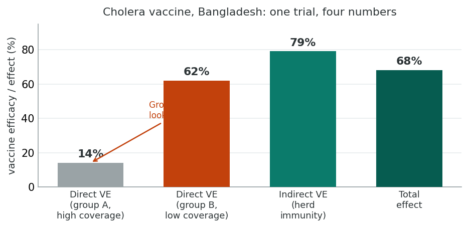
Designing Vaccine Trials to Estimate All Three Measures
To estimate VEd, VEind, and VEtot, the design must include at least two comparable populations with different vaccination coverage. The recommended approach: in population A, randomise individuals to vaccine or placebo. In population B, leave everyone unvaccinated (or assign a lower coverage). The two populations must be (a) comparable in characteristics that affect the outcome, especially baseline transmission level, and (b) physically separated so subjects do not intermix.
An alternative when finding two similar populations is impractical is to exploit natural clustering, for example randomly assigning vaccination to half the children in a geographic area, then study spread within schools, recording the proportion of children at each school who were vaccinated. Riggs and Koopman (2005) and Longini and colleagues (1998, 2002) describe how to design and analyse such trials.
Reporting: The CONSORT 2025 Checklist
A later lesson (Integrated Appraisal of Epidemiological Research) introduces CONSORT's key requirements and its flow diagram as a framework for appraising published trials. CONSORT 2025 (Hopewell et al., 2025) is the dominant reporting guideline for parallel-group randomised trials. It updates CONSORT 2010, replacing its 25 items with 30 and adding a section on open science (registration, protocol, data sharing, funding and conflicts of interest). Its items align with the design and conduct topics covered in this and the previous two sections; the table below highlights those most relevant to the topics we have studied, numbered as in the 2025 checklist.
| Section / Item | What to Report |
|---|---|
| 1a Title | Identify the study as a randomised trial in the title (improves “searchability”). |
| 2–5 Open science | Trial registration; where the protocol and statistical analysis plan can be accessed; how data and code can be accessed; funding and conflicts of interest. |
| 6–7 Background & objectives | Scientific rationale and specific objectives about benefits and harms. |
| 8 Patient and public involvement | How patients or the public were involved in the design, conduct and reporting of the trial. |
| 9 Trial design | Type of design (parallel, factorial, cross-over, cluster, split-plot), allocation ratio, and framework (superiority, equivalence, non-inferiority). |
| 11–12 Setting & eligibility | Settings and locations; eligibility criteria for participants and, if applicable, for sites and those delivering the interventions. |
| 13 Intervention & comparator | Sufficient detail for replication, including how and when administered. |
| 14–15 Outcomes & harms | Pre-specified primary and secondary outcomes and how they were assessed; how harms were defined and assessed. |
| 16a–b Sample size | How sample size was determined; explanation of any interim analyses or stopping guidelines. |
| 17–19 Randomisation | How the allocation sequence was generated, what type of restriction (blocking) was used, the mechanism for concealing allocation, and whether those enrolling participants had access to the sequence. |
| 20a–b Blinding | Who was blinded after assignment (participants, providers, outcome assessors); how blinding was achieved and the similarity of interventions. |
| 21a–d Statistical methods | Methods for primary and secondary outcomes and harms; who was included in each analysis; how missing data were handled; subgroup and sensitivity analyses. |
| 22a–b Participant flow | For each group, numbers randomly assigned, receiving intended treatment, and analysed for the primary outcome; losses and exclusions with reasons. A flow diagram is strongly recommended. |
| 23a–b Recruitment | Dates of recruitment and follow-up; reasons the trial ended or was stopped. |
| 24a–b Intervention delivery | The intervention and comparator as actually delivered, including adherence, and any concomitant care. |
| 25 Baseline data | Table of baseline demographic and clinical characteristics for each group. |
| 26 Numbers analysed, outcomes & estimation | For each group, the numbers analysed; effect size and precision (e.g., 95% CI); for binary outcomes, both absolute and relative effect sizes. |
| 27 Harms | All harms or unintended events in each group. |
| 28 Ancillary analyses | Other analyses (subgroup, sensitivity), distinguishing pre-specified from post hoc. |
| 29–30 Discussion | Interpretation balanced against benefits and harms and other evidence; limitations (bias, imprecision, generalisability, multiplicity). |
CONSORT extensions exist for cluster randomised trials, non-inferiority and equivalence trials, non-pharmacological treatments, herbal interventions, and pragmatic trials. They were developed for CONSORT 2010 and are used alongside the current statement until they are updated. Up-to-date references are available at www.consort-statement.org.
Key Takeaways
- Rigorous and equal follow-up of all groups is essential. Document compliance and reasons for withdrawal; a CONSORT flow diagram is strongly recommended.
- Intent-to-treat analysis preserves randomisation and gives a conservative, real-world estimate; per-protocol analysis estimates the effect under ideal compliance and should be reported alongside ITT, not in place of it.
- Multiple comparisons inflate the experiment-wise error rate. The Bonferroni adjustment (α / k) is the simplest correction. Subgroup analyses should be pre-specified and tested via interaction terms; data-driven subgroup analyses generate spurious findings.
- For prophylactic vaccines, three measures matter: direct (VEd), indirect or herd-immunity (VEind), and total (VEtot) efficacy. Estimating all three requires data from at least two populations with different coverage.
- The CONSORT 2025 checklist of 30 items, which updates CONSORT 2010, structures both the planning and the reporting of randomised trials. Following CONSORT from the design stage through to write-up is what makes transparent reporting achievable.
The reflection below asks you to design a trial of your own, drawing on all three trial sections. After working through it and the knowledge check, the final assessment draws on all seven sections of the lesson.
Reflection
Reflection
Imagine you have been funded to design a randomised controlled trial of a new mobile-app-based behavioural intervention to reduce daily smoking among young adults aged 18–25 living in rural communities. Briefly outline how you would address: (1) the target population (the group to which you want to generalise), the source population (the accessible group from which participants are recruited), and the study sample (the participants actually enrolled); (2) the choice of allocation strategy (individual randomisation; cluster randomisation, in which whole communities or clinics are assigned together; or a factorial design, which tests two interventions at once); (3) the choice of comparator (no app, a sham app, or existing standard care); and (4) how you would handle the analysis if compliance with the app turned out to be poor, noting that intention-to-treat analysis keeps participants in the group to which they were assigned, while per-protocol analysis includes only those who complied. Identify at least one trade-off you would face and explain how you would resolve it.
Minimum 20 characters required.
1. The major reason that intent-to-treat analysis is preferred as the primary analysis is that:
2. In a vaccine trial, the indirect vaccine efficacy (VEind) is estimated by:
3. With four pre-specified primary outcome comparisons and a desired family-wise error rate of 0.05, the Bonferroni-adjusted significance threshold for each comparison is:
4. The CONSORT 2025 statement is:
Final Review & Assessment
⏱ Estimated time: 30 minutes
Bringing It All Together
Where an earlier lesson looked backward from outcome to exposure, this lesson followed the arrow forward. An earlier section framed the cohort study as something close to a controlled trial without randomisation: pick a source population, classify exposure, follow people, and watch incidence accumulate. An earlier section then forced the central design choice, risk-based (cumulative incidence) for closed populations followed for a fixed time, or rate-based (incidence density) for open populations where person-time is the natural denominator, and connected each to its analytic toolkit (binomial / log-binomial vs. Poisson / survival).
Earlier sections zoomed in on the operational details that decide whether a cohort study survives appraisal. How exposure is scaled (dichotomous, ordinal, continuous, compound), whether it changes over time, how the induction period is handled, and how comparability is engineered through restriction, matching, and analytic control all determine whether the rate ratio you eventually report is estimating what you think it is. Blinded outcome ascertainment, careful handling of loss to follow-up, and STROBE-aligned reporting then turn a defensible design into a study other researchers can actually use.
The last three sections crossed from observational into experimental epidemiology. They set out the rationale for randomised controlled trials, the phases of clinical research, the mechanics of allocation and masking, sample size with the inflation factor for cluster trials, and the analytic and reporting standards (intention-to-treat, CONSORT 2025) that govern modern trial conduct. The shift is conceptually small, since the investigator now assigns the exposure that a cohort study can only classify, but methodologically large, because randomisation is what gives trials their causal authority.
The final reflection asks you to put the entire arc to work as a brief cohort proposal of your own; the 24-question assessment then checks the conceptual content of all seven sections directly. A later lesson will pull the camera back further to look at ecological and group-level designs (where the unit of analysis stops being the person) and the comparability and inference logic you just built will keep paying off there.
Key Takeaways from this lesson
- Cohort studies follow exposed and unexposed people forward in time, giving you direct access to incidence, something case-control studies cannot deliver.
- The choice between risk-based (closed cohort, cumulative incidence) and rate-based (open cohort, incidence density) designs is dictated by the source population and the follow-up structure, not by preference.
- Person-time is the right denominator whenever follow-up is uneven or membership is dynamic; it makes Poisson and survival analyses possible.
- Exposure must be measured on a meaningful scale, with explicit handling of induction periods and time-varying status, misclassification here flows through the whole analysis.
- Comparability is engineered through restriction, matching, and analytic control; blinded outcome ascertainment and rigorous tracking of loss-to-follow-up protect internal validity.
- STROBE-aligned reporting closes the loop: a cohort study is only as useful as its design, conduct, and analysis are visible to the reader.
- Randomisation is what makes the RCT the gold standard for causal inference about interventions: it balances measured and unmeasured confounders in expectation, and trial design begins with explicit target, source, and study populations and a precisely specified intervention.
- Allocation strategies (simple, stratified, cross-over, factorial, cluster, split-plot, multicentre) and masking (single, double, triple) each prevent specific biases; cluster trials must inflate sample size by the design effect, DEFF = 1 + (m − 1) × ICC.
- Intention-to-treat is the primary analysis because it preserves randomisation; vaccine trials distinguish direct, indirect, and total efficacy; and the CONSORT 2025 checklist structures both planning and reporting.
Reflection
Design a brief cohort study proposal for a health question of your choice. Specify: (1) the research question and hypothesis, (2) whether the source population is open or closed, (3) whether you would use a risk-based or rate-based design and why, (4) how you would define and measure exposure (and on what scale), (5) how you would ensure comparability of groups, and (6) what analytic approach you would use.
Minimum 20 characters required.
Final Knowledge Assessment
This assessment covers all sections of this lesson. You must score 100% to complete the lesson. Review the feedback after each attempt.
1. The fundamental logic of a cohort study is to:
2. A cohort study most resembles which other design?
3. In a closed source population, all subjects:
4. In a risk-based cohort study, what is the denominator of the risk?
5. In a rate-based cohort study, the denominator is:
6. Which design is best suited for studying a chronic disease with a long, lifelong risk period?
7. Which is an example of a compound exposure variable?
8. The induction period is:
9. If a subject’s exposure status changes during follow-up:
10. Which approach to comparability is applied during analysis rather than design?
11. Which statement about exchangeability in observational studies is correct?
12. Why are incident cases preferred over prevalent cases for cohort outcomes?
13. For a rate-based cohort study where rates can be assumed reasonably constant, which model is appropriate?
14. Hernan (2010) describes which problem with the average hazard ratio?
15. According to STROBE-style criteria for cohort studies, which item should be reported?
16. Randomising participants between a new treatment and a comparator is ethically defensible only when:
17. A drug has been licensed and is now being monitored in very large patient populations over long periods to detect rare or slow-to-appear adverse effects. This stage of clinical research is:
18. Compared with broad eligibility criteria, narrow eligibility criteria in a trial generally:
19. In a cluster randomised trial of a school-based health programme with intracluster correlation coefficient ICC = 0.02 and an average cluster size of 51 students per school, the sample-size inflation factor is:
20. Triple-blinding adds which additional layer of masking compared with double-blinding?
21. The CAESAR trial randomised women having a first Caesarean section to single- or double-layer uterine closure, to closure or non-closure of the peritoneum, and to liberal or restricted use of a drain, with every combination possible. This allocation design is a:
22. The recommended primary analysis for a randomised controlled trial is:
23. In the Bangladesh cholera vaccine trial, direct vaccine efficacy was only 0.14 in the high-coverage population but 0.62 in the low-coverage population. The best explanation is that:
24. Investigators want to know whether a trial's treatment effect differs between men and women. The recommended approach is to: