Mediation, Moderation and Path Analysis
Exploratory Data Analysis For Epidemiology
Learning objectives for this lesson:
- Use a DAG to distinguish a confounder, a mediator and a collider, explain why effect modification is a separate question that a standard DAG does not encode, and state the research question each role implies.
- Define total, direct and indirect effects, and state the assumptions required to interpret an indirect effect causally, including temporal order and the absence of unmeasured mediator-outcome confounding.
- Specify, fit and interpret a regression model with an interaction term, compute and plot simple slopes, and explain the role of centring.
- Estimate an indirect effect by the product-of-coefficients and difference methods, explain the limits of the Baron and Kenny steps, and obtain a bootstrap confidence interval with the
mediationpackage. - Draw a path diagram, specify it in lavaan syntax, estimate direct and indirect paths, and compare nested path models.
- Explain how path analysis with observed variables extends to structural equation modelling with latent variables, building on the confirmatory factor analysis in Lesson 7.
- Report mediation and moderation results in text, tables and figures without causal overstatement.
This course was developed by Dr. Kiffer G. Card, Faculty of Health Sciences, Simon Fraser University based on Dohoo, I. R., Martin, S. W., & Stryhn, H. (2012). Methods in Epidemiologic Research. VER Inc.
Glossary: Key Terms, People & Concepts
📚 Reference page, available throughout the lesson
This glossary collects the key concepts, methods and people in this lesson. It can be used as a reference while working through the material or as a review before assessments. Typing in the search box filters the entries.
mediate(). In cross-sectional data they are statistical quantities despite their names.
medsens() reports the correlation ρ between the residuals of the mediator and outcome models at which the indirect effect would fall to zero.
~ for regressions, ~~ for covariances, =~ for latent variables and := for defined quantities such as an indirect effect.
mediation package and its sensitivity analysis.
What Role Does the Third Variable Play?
The CSCS 2021 data
Introduction and Overview
This is the last lesson of HSCI 410. It continues the loneliness thread from Lesson 7, Measurement and Psychometrics, which asked how well loneliness and related constructs are measured. This lesson asks how such measures relate to one another. Most models in the course so far have related one exposure to one outcome, with other variables added as adjustments. Many research questions are about a third variable in its own right: whether it explains part of an association, or whether an association is stronger in some groups than in others. These are questions of mediation and moderation, and the last section of the lesson shows how both can be written as a path model. This first section sets out the roles a third variable can play, defines the effects that mediation analysis estimates, and states the conditions under which those effects can be read causally.
Learning Objectives
- Use a DAG to distinguish a confounder, a mediator and a collider, explain why effect modification is a separate question that a standard DAG does not encode, and state the research question each role implies.
- Define the total, direct and indirect effects, and explain how they are related in a linear model.
- State the assumptions required to interpret an indirect effect causally, including temporal order and the absence of unmeasured mediator-outcome confounding.
- Explain why cross-sectional data support only statistical mediation, and describe a mediation result without causal overstatement.
- Load and prepare the CSCS 2021 variables used throughout the lesson in R.
The section begins with the practical problem that motivates the whole lesson and then turns to the causal diagram that classifies each variable in it.
The Running Case: Two Questions from a Community Connector Program
The methods in this lesson are easier to follow when they answer a concrete question. Box 8.1 describes a community connector program whose staff have two questions about social support, loneliness, depressive symptoms and age, and it names the survey that the analyst uses to explore them. The same case and the same survey are used in every section of the lesson.
A community connector program links adults who are isolated or under strain with local groups, volunteers and services. Its staff believe that the support people gain through the program protects their mental health, and they suspect that it does so partly by making people less lonely. They also wonder whether the program matters more for older participants. Before designing an evaluation, they ask an analyst two questions that can be explored in existing data. First, is social support associated with fewer depressive symptoms partly because people with more support are less lonely? Second, is the association between social support and loneliness the same for younger and older adults?
The analyst turns to the 2021 wave of the Canadian Social Connection Survey (CSCS), the dataset used in the narrated R walkthroughs. It contains a social support score (the Multidimensional Scale of Perceived Social Support; Zimet et al., 1988), a loneliness score (the three-item UCLA Loneliness Scale; Hughes et al., 2004), a depressive symptom score (the two-item Patient Health Questionnaire, PHQ-2; Kroenke et al., 2003) and age. In the 2021 wave, 3,110 people answered all four questions.
The first question is a mediation question, because loneliness is proposed as a step on the pathway from support to depressive symptoms. The second is a moderation question, because age is proposed as a variable that changes the size of an association. The same three variables appear in both, yet the analyses differ, because the third variable plays a different role in each. Identifying that role is the first step of the analysis.
Three DAG Positions, and Effect Modification as a Separate Question
A causal diagram is the tool that identifies the role of a third variable. This part recalls the directed acyclic graph from Lesson 1, uses it to define the confounder, the mediator and the collider, and explains why effect modification is a separate question that the diagram does not encode. Box 8.2 recalls the elements of a DAG and poses a retrieval question about colliders.
Box 8.2: Recall: Lesson 1, Section 1 (Start with a Causal Diagram)
Lesson 1, Section 1 introduced the directed acyclic graph (DAG), in which each variable is a node, each assumed causal effect is an arrow, and no variable can cause itself through a loop. Its arrows record the analyst's assumptions, which come from theory and earlier research (Greenland, Pearl and Robins, 1999). Lesson 1 named three structures: a fork (X ← C → Y), in which C is a confounder; a chain (X → M → Y), in which M is a mediator; and a collider (X → Z ← Y).
Retrieval question. What happens when an analysis adjusts for, or selects the sample on, a collider Z of X and Y?
With an exposure X and an outcome Y in place, a DAG distinguishes three positions for a third variable: confounder, mediator and collider. Effect modification is a separate question about the size of the X to Y effect across levels of a variable V. A standard DAG does not encode it, because an arrow states only that an effect exists, so it is shown by a note on the diagram or by drawing the diagram within each stratum of V. Figure 8.1 shows the three positions and, in panel D, effect modification drawn within strata.
The cards below describe the three positions and effect modification, the research question each implies and what it asks of the analysis.
Table 8.1 brings the four roles together in one place. For each role it gives the position in the DAG, the research question the role implies and what the analysis does with the variable.
Table 8.1. The four roles a third variable can play, the research question each implies and what the analysis does.
| Role | Position in the DAG | Research question it implies | What the analysis does |
|---|---|---|---|
| Confounder (C) | X ← C → Y | Is X associated with Y when C is held constant? | Adjusts for C. |
| Mediator (M) | X → M → Y | How much of the X to Y association runs through M? | Splits the total into direct and indirect parts. |
| Collider (Z) | X → Z ← Y | None; Z is a consequence of X and Y. | Leaves Z out of the model and does not select on it. In the referral example the collider is selection into the sample (S). |
| Effect modifier (V) | Not a DAG position; shown by a note or by drawing the DAG within each stratum of V | Does the X to Y association differ across levels of V? | Fits an X × V interaction or stratifies by V. |
Two of these roles are easily confused in practice, because a mediator and a confounder look alike in the data. Box 8.3 explains how the direction of one arrow separates them.
⚠ Box 8.3: Mediator or confounder
A mediator and a confounder are both associated with the exposure and with the outcome, so they cannot be told apart from correlations alone. The difference lies in the direction of the arrow between the exposure and the third variable. A confounder affects the exposure, and the analysis adjusts for it. A mediator is affected by the exposure, and adjusting for it when the total effect is the target removes part of the association that the study set out to estimate. Deciding which arrow is more plausible requires subject knowledge about timing and mechanism, and in some studies a variable could play either role.
Sort the roles
Each scenario below names an exposure, an outcome and a third variable. Choose the DAG position the third variable takes (confounder, mediator or collider), or choose effect modifier when the scenario is about the size of the association, which a DAG does not show. Feedback appears after each choice.
Interactive 8.1 gives practice in the distinctions drawn in Table 8.1 and Box 8.3. It presents eight scenarios, five built on the running case and three from other areas of public health.
📊 Interactive 8.1: Role sorter: eight scenarios
1. Exposure: social support. Outcome: depressive symptoms. Third variable: a long-term health condition, which can limit social contact and can also raise depressive symptoms.
2. Exposure: social support. Outcome: depressive symptoms. Third variable: loneliness, which may fall when support rises and may in turn lower depressive symptoms.
3. Exposure: social support. Outcome: loneliness. Third variable: age group, because the association appears stronger among adults aged 50 and over than among younger adults.
4. Exposure: social support. Outcome: depressive symptoms. Third variable: referral to the program, which is more likely for people with low support and for people with depressive symptoms. The analysis includes referred people only.
5. Exposure: social support. Outcome: depressive symptoms. Third variable: household income, which affects the time and resources people have for social contact and also affects mental health through financial strain.
6. Exposure: joining a walking group. Outcome: blood pressure six months later. Third variable: weekly minutes of physical activity at three months.
7. Exposure: a smoking cessation program. Outcome: quitting at one year. Third variable: living with a partner who does not smoke, because the program appears to work better for people who do.
8. Exposure: severe infection. Outcome: frailty. Third variable: hospital admission, which is more likely for people with a severe infection and for people who are frail. A study of admitted patients only finds that infection and frailty are negatively associated.
The DAG has now fixed the role of each third variable in the running case. Loneliness is the proposed mediator of the association between support and depressive symptoms, and age is a proposed effect modifier of the association between support and loneliness. The next part takes the mediator and shows how the association it carries can be divided.
Total, Direct and Indirect Effects
Once loneliness has been identified as a proposed mediator, the association between support and depressive symptoms can be divided into parts. The total effect is the association between the exposure and the outcome when the mediator is ignored. The indirect effect is the part of the total that runs through the mediator. The direct effect is the part that remains when the mediator is held constant, which includes every pathway the model does not name. The word "effect" is the conventional statistical name for these quantities. In cross-sectional data such as the CSCS, each one is an association, and it describes a cause only under the assumptions set out later in this section.
Mediation analysis labels the paths with letters. Path a runs from the exposure to the mediator. Path b runs from the mediator to the outcome, with the exposure held constant. Path c is the total effect, and path c′ (read "c prime") is the direct effect.
Figure 8.2 draws these paths for the running case, with the total effect in the upper diagram and its division into direct and indirect parts in the lower one.
When the mediator and the outcome are continuous and every model is a linear regression fitted to the same people, the parts add up exactly.
Equation 8.1 expresses this decomposition in the path labels of Figure 8.2.
The causal-inference literature defines these quantities more generally with counterfactuals: the indirect effect is the change in the outcome that would follow if the mediator shifted from the value it would take at one level of the exposure to the value it would take at another, with the exposure itself held fixed (Robins and Greenland, 1992; Pearl, 2001). These definitions do not depend on a particular model, and they are the basis of the mediate() function used in Section 3. For linear models without interactions, they give the same numbers as a × b and c′.
The decomposition in Equation 8.1 is arithmetic, and it holds in any dataset in which the linear models are fitted to the same people. Whether the indirect part describes a causal pathway is a separate matter, which depends on the conditions set out in the next part.
Conditions for Reading an Indirect Effect Causally
An estimated indirect effect describes a causal pathway only if several conditions hold (VanderWeele, 2015). None of them can be confirmed from the data alone, which is why the DAG and the study design carry so much of the argument.
The accordion below lists the five conditions, with one panel for each condition.
The exposure must occur before the mediator, and the mediator before the outcome. A cohort that measures support at one visit, loneliness at a later visit and depressive symptoms later still provides this order. A single survey that asks about all three at once does not.
Every common cause of the exposure and the outcome must be measured and adjusted for. This is the same condition that any estimate of a total effect requires.
Every common cause of the exposure and the mediator must be measured and adjusted for, so that path a describes the effect of the exposure on the mediator.
Every common cause of the mediator and the outcome must be measured and adjusted for. This condition is the easiest to overlook, because randomizing the exposure does not satisfy it. In a trial that assigns people to the community connector program at random, loneliness is still not assigned at random. A history of depression, for example, could raise both loneliness and later depressive symptoms. When such a variable is left out, the estimate of path b is biased, and so are the direct and indirect effects (Cole and Hernán, 2002).
No common cause of the mediator and the outcome may itself be caused by the exposure. If support affects physical activity, and physical activity affects both loneliness and depressive symptoms, the usual direct and indirect effects cannot be separated by regression adjustment alone.
Box 8.4 describes how careful mediation analyses respond to the fourth condition.
Box 8.4: Sensitivity analysis
Because the fourth condition cannot be checked, careful mediation analyses report how strong an unmeasured mediator-outcome confounder would need to be to remove the indirect effect. Section 3 runs this sensitivity analysis with the medsens() function of the mediation package.
The first condition, temporal order, is a matter of study design, and it is a condition that the CSCS data cannot meet. The next part explains why, and what kind of conclusion the data can still support.
Cross-Sectional Data Support Statistical Mediation Only
The CSCS 2021 wave measured social support, loneliness and depressive symptoms in the same survey, at the same time. The first condition, temporal order, therefore cannot be established. Each arrow in the mediation diagram could plausibly run in the other direction. People with depressive symptoms may withdraw from others and feel lonelier, and they may also perceive the support around them as weaker than others would judge it. Maxwell and Cole (2007) showed that mediation estimates from cross-sectional data can differ substantially from the longitudinal processes they are meant to describe.
The analysis in this lesson is still informative. It shows whether the pattern of associations is consistent with the program's explanation, and how large the indirect association is. That information can justify a longitudinal evaluation of the program. It is reported as a statistical decomposition of an association, and causal language is kept for designs in which the conditions above are plausible.
Table 8.2 sets the two kinds of wording side by side, using the CSCS results that Section 3 estimates. The left column describes a statistical decomposition, and the right column claims a causal pathway that the data cannot show.
Table 8.2. Wording suited to a cross-sectional mediation result, set against wording that claims a causal pathway.
| Wording suited to cross-sectional data | Wording that claims a causal pathway |
|---|---|
| Loneliness statistically accounted for about 41% of the association between social support and depressive symptoms. | Social support reduced depressive symptoms by reducing loneliness. |
| The indirect association through loneliness was −0.23 PHQ-2 points per point of support. | Each extra point of support caused a 0.23-point fall in depressive symptoms through loneliness. |
| The pattern of associations is consistent with a pathway through loneliness, which a longitudinal study could test. | Loneliness is the mechanism by which support protects mental health. |
The analyses in this lesson are therefore reported as statistical decompositions of associations in the CSCS. The last part of this section loads those data in R and describes the three variables.
Meeting the Data
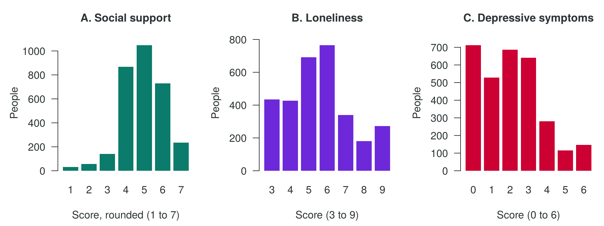
Activity 8.1 loads the CSCS data and prepares the variables with the same code as the narrated walkthrough Mediation and Moderation, so that every number in this lesson can be reproduced. Figure 8.3 shows the three scores for the 3,110 people with complete data. Support is concentrated between 4 and 6 on its 1 to 7 scale, loneliness spreads across its 3 to 9 range, and depressive symptoms are most often between 0 and 3 on the 0 to 6 PHQ-2 scale.
This activity loads the 2021 wave of the CSCS and prepares the variables used throughout the lesson. The data are read directly from GitHub, so no file needs to be downloaded, although the first line takes a few seconds to run. The code is the same as in the narrated walkthrough, which shows each step in more detail.
# Load the CSCS data from GitHub (this takes a few seconds)
github_url <- "https://raw.githubusercontent.com/jorgeandr3s/heal/main/cscs/public_data/CSCS2025_full_cleaned_deidentified_data_and_metadata.RData"
load(url(github_url))                                 # creates a data frame called data
data <- data[data$SURVEY_collection_year == 2021, ]   # keep the 2021 wave
dim(data) # people (rows) and variables (columns)The 2021 wave holds 4,045 people (rows) and 3,247 variables (columns). The data[ , ] line keeps the rows whose survey year is 2021, so that each person appears once.
# support:    social support (MSPSS), 1 to 7, higher = more support
# loneliness: UCLA 3-item Loneliness Scale, 3 to 9, higher = lonelier
# depression: PHQ-2 depressive symptoms, 0 to 6, higher = more symptoms
med_data <- data.frame(
  support    = data$PSYCH_zimet_multidimensional_social_support_scale_score,
  loneliness = data$LONELY_ucla_loneliness_scale_score,
  depression = data$WELLNESS_phq_score,
  age        = data$DEMO_age)
summary(med_data)The data.frame() call copies four variables into a small data frame with short names. The summary shows a mean support score of 4.93, a mean loneliness score of 5.58 and a mean depressive symptom score of 2.07. The NA's row counts missing answers: 829 for support, 462 for loneliness and 743 for depressive symptoms. Age has no missing values.
med_data <- na.omit(med_data)   # keep people with no missing values
nrow(med_data)                  # how many people are in the analysis?
round(cor(med_data[, c("support", "loneliness", "depression")]), 2)Reading the output. na.omit() keeps the 3,110 people who answered all four questions, so that every model in the lesson uses the same people. In the correlation matrix, support is negatively correlated with loneliness (−0.40) and with depressive symptoms (−0.38), and loneliness is positively correlated with depressive symptoms (0.47). These signs fit the program's proposed pathway, in which more support goes with less loneliness and less loneliness goes with fewer symptoms, but correlations cannot show the direction of any arrow.
R Reflect on what you just ran
Use the questions below to interpret the output you produced. Look at your console output before answering.
1. How many people are in the analysis after na.omit(), and why does every model in the lesson need to use the same people?
2. Report the three correlations and describe what their signs mean for the community connector program's proposed pathway.
3. The correlations would look the same if depressive symptoms led to lower perceived support and to more loneliness. Explain why, and what kind of data would help to separate these explanations.
This section has identified the role of each third variable in the running case, defined the total, direct and indirect effects, stated the conditions for a causal reading, and prepared the 3,110 complete cases in R. Section 2 takes up the second question of the running case, whether the association between support and loneliness differs by age. The knowledge check that follows covers the material of this section.
1. In the community connector question, loneliness is proposed as a variable that is lowered by social support and that in turn lowers depressive symptoms. Which role does loneliness play?
2. Why should a mediator be left out of a model whose aim is to estimate the total effect of an exposure?
3. A study of people referred to a support program finds that, among them, low social support and depressive symptoms are unrelated, although both raise the chance of referral. What is the most likely problem?
4. In a linear mediation analysis fitted to the same people, the total effect is c = −0.50 and the direct effect is c′ = −0.30. What is the indirect effect by the difference method?
5. Why do the CSCS 2021 data support only a statistical decomposition of the association between support and depressive symptoms?
✎ Reflection
A researcher is studying whether regular volunteering (the exposure) is associated with better self-rated health (the outcome) among adults aged 60 and over. She has four other variables: (1) household income, which affects both the chance of volunteering and health; (2) physical activity, which volunteering is thought to increase and which is thought to improve health; (3) whether the person was recruited through a volunteer centre, which is more likely for people who volunteer and for people in good health; and (4) gender, because the association appears stronger in women than in men. In this lesson, a confounder causes both the exposure and the outcome, a mediator lies on the pathway from the exposure to the outcome, a collider is caused by both the exposure and the outcome, and an effect modifier changes the size of the association. For each of the four variables, name its role, state the research question it implies, and say what the analysis should do with it. Then explain why a cross-sectional survey would allow only a statistical description of the pathway through physical activity.
Moderation: When an Association Differs Across Groups
A steeper slope for adults aged 50 and over
The support slope at ages 30, 50 and 70
Introduction
The second question from the community connector program asks whether the association between social support and loneliness is the same for younger and older adults. This is a question of moderation. A moderator is a variable across whose levels the association between an exposure and an outcome differs in size or direction. Epidemiologists usually call the same idea effect modification, a term met in HSCI 341, and psychologists usually call it moderation. Lesson 3 showed the mechanics of adding an interaction term to a regression. This section treats moderation as a research question: what the interaction coefficient means, how to read the other coefficients when an interaction is present, and how to present the result.
Learning Objectives
- Distinguish a moderation question from a confounding question and from a mediation question.
- Specify, fit and interpret a linear regression with an interaction between a continuous exposure and a binary moderator.
- Explain what the main effects mean when an interaction is present, and why centring a continuous moderator helps.
- Compute and plot simple slopes at chosen values of a moderator.
- Explain the difference between interaction on the additive and multiplicative scales.
The section first separates moderation from confounding and mediation. It then writes the interaction model, fits it to the CSCS data with age in two groups and as a continuous variable, and closes with the scale of an interaction and the reporting of a moderation result.
Moderation as a Research Question
Moderation asks for whom or under what conditions an association is stronger or weaker. Mediation, the topic of Section 3, asks why an association exists. The two can involve the same variables, but they are different questions with different models. A third question, confounding, asks whether an association remains once a common cause is held constant.
Table 8.3 poses one question of each type about age in the running case and shows the model that answers each one in R.
Table 8.3. Three questions about age in the running case, with the type of question, the model in R and what the model gives.
| Question about age | Type | Model in R | What the model gives |
|---|---|---|---|
| Is support associated with loneliness once age is held constant? | Confounding | lm(loneliness ~ support + age_group) | One support slope for everyone, adjusted for age. |
| Is the support slope different for adults aged 50 and over? | Moderation | lm(loneliness ~ support * age_group) | A support slope for each age group and a test of the difference. |
| Does a third variable carry part of the association from support to depressive symptoms? | Mediation | Several models (Section 3) | A direct part and an indirect part. |
The models in the first two rows of Table 8.3 both contain age, and they differ by one term. Box 8.5 explains why adjusting for age leaves the moderation question untested.
⚠ Box 8.5: Adjusting for a variable does not test whether it modifies an association
Adding age to a model as a covariate adjusts the support coefficient for age. The model still estimates a single slope for support, which is assumed to be the same at every age, and it contains no test of whether the slope differs. Testing moderation requires a term that allows the slope to change with age, which is the interaction term. A variable can be a confounder, a moderator, both or neither, and each role is checked with a different model.
A moderation question therefore needs a model in which the slope of support can change with age. The next part writes that model and explains each of its coefficients.
The Interaction Model
For the running case, the moderator is an indicator called older, equal to 1 for adults aged 50 and over and 0 for adults under 50 (the reference group). The interaction model adds the product of support and the indicator to a model that already contains both.
Equation 8.2 writes the model with four coefficients, and the explanation under it shows how the model reduces to one line for each age group.
In R, support * age_group is shorthand for support + age_group + support:age_group, so the main effects are included automatically. Table 8.4 gives the meaning of each coefficient.
Table 8.4. The four coefficients of Equation 8.2, their names in the R output and their meaning.
| Coefficient | Name in R output | Meaning |
|---|---|---|
| β0 | (Intercept) | Predicted loneliness for an adult under 50 with a support score of 0. |
| β1 | support | Slope of support among adults under 50 (the reference group) only. |
| β2 | age_group50 and over | Difference in predicted loneliness between the age groups at a support score of 0. |
| β3 | support:age_group50 and over | Difference between the support slope at 50 and over and the support slope under 50. |
With the meaning of each coefficient fixed, the model can be fitted to the CSCS data. The next part does so with age in two groups.
Moderation by Age Group in the CSCS
Activity 8.2 creates the two age groups, fits the models without and with the interaction, compares them, and calculates the slope of support in each group. Of the 3,110 people, 2,275 are under 50 and 835 are aged 50 and over.
This activity uses the same data and preparation as Section 1 and adds the moderator. The first lines load and prepare the data again, so the activity can be run on its own. The age groups are made with the bracket recoding pattern from the data cleaning walkthrough.
github_url <- "https://raw.githubusercontent.com/jorgeandr3s/heal/main/cscs/public_data/CSCS2025_full_cleaned_deidentified_data_and_metadata.RData"
load(url(github_url))                                 # creates a data frame called data
data <- data[data$SURVEY_collection_year == 2021, ]   # keep the 2021 wave
med_data <- data.frame(
  support    = data$PSYCH_zimet_multidimensional_social_support_scale_score,
  loneliness = data$LONELY_ucla_loneliness_scale_score,
  depression = data$WELLNESS_phq_score,
  age        = data$DEMO_age)
med_data <- na.omit(med_data)   # the same people in every model
# The moderator: two age groups, with "Under 50" as the reference
med_data$age_group <- NA
med_data$age_group[med_data$age < 50] <- "Under 50"
med_data$age_group[med_data$age >= 50] <- "50 and over"
med_data$age_group <- factor(med_data$age_group,
                             levels = c("Under 50", "50 and over"))
table(med_data$age_group)The table confirms 2,275 adults under 50 and 835 adults aged 50 and over. Setting levels in factor() makes "Under 50" the reference group.
# support * age_group is shorthand for
# support + age_group + support:age_group
model_main <- lm(loneliness ~ support + age_group, data = med_data)
model_int  <- lm(loneliness ~ support * age_group, data = med_data)
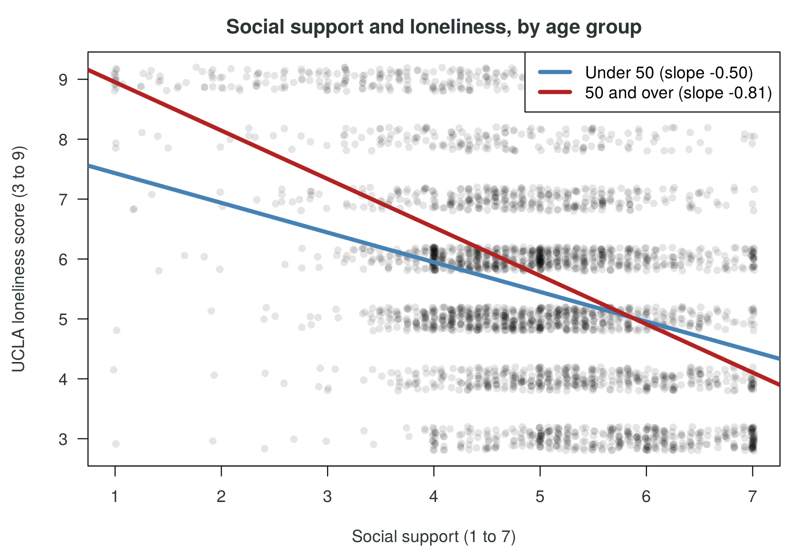
summary(model_int)Reading the output. The support coefficient (−0.495) is the support slope among adults under 50. The interaction coefficient support:age_group50 and over (−0.312, p = 2.1 × 10⁻⁹) is the difference between the slopes, so the slope among adults aged 50 and over is −0.495 + (−0.312) = −0.808. The age_group50 and over coefficient (1.83) compares the groups at a support score of 0, outside the 1 to 7 scale. Together, the three predictors explain about 18% of the variation in loneliness (R-squared 0.177).
anova(model_main, model_int) # does the interaction improve the model?The comparison tests whether adding the interaction improves the model. The F statistic is 36.1 on 1 degree of freedom (p = 2.1 × 10⁻⁹), the same p-value as the t test of the interaction coefficient, because the models differ by one term.
# Simple slopes: the slope of support in each age group
coef(model_int)["support"]                                     # Under 50
coef(model_int)["support"] + coef(model_int)["support:age_group50 and over"] # 50 and overThe simple slopes are −0.495 under 50 and −0.808 at 50 and over. R keeps the name support on the second number because it is the first coefficient in the sum.
# One fitted line for each age group
plot(jitter(med_data$support), jitter(med_data$loneliness),
     xlab = "Social support (1 to 7)", ylab = "UCLA loneliness score (3 to 9)",
     pch = 16, col = rgb(0, 0, 0, 0.10))
abline(lm(loneliness ~ support,
          data = med_data[med_data$age_group == "Under 50", ]),
       col = "steelblue", lwd = 3)
abline(lm(loneliness ~ support,
          data = med_data[med_data$age_group == "50 and over", ]),
       col = "firebrick", lwd = 3)
legend("topright", legend = c("Under 50", "50 and over"),
       col = c("steelblue", "firebrick"), lwd = 3)
This code produces no console output. It draws the scatterplot with one fitted line per age group shown in Figure 8.4. jitter() adds a small random amount to each value so that people with the same scores do not hide behind one another.
R Reflect on what you just ran
Use the questions below to interpret the output you produced. Look at your console output and plots before answering.
1. Report the interaction coefficient with its p-value, and explain in one or two sentences what it says about the two age groups.
2. Give the simple slope of support in each age group and interpret each one in a sentence that describes an association.
3. A colleague writes that "being 50 or over raises loneliness by 1.83 points". Explain why this reading of the age_group50 and over coefficient is wrong.
Figure 8.4 shows the plot that the last chunk of code in Activity 8.2 draws. The two fitted lines make the interaction visible, because the line for adults aged 50 and over is the steeper of the two.
Reading the main effects when an interaction is present
Once an interaction term is in the model, each main effect describes a slope or a difference at the zero point of the other variable. The support coefficient (−0.50) is the support slope for adults under 50, and it applies to no one else. The age_group50 and over coefficient (1.83) is the difference between the age groups at a support score of 0. The support scale runs from 1 to 7, so a score of 0 is impossible, and this coefficient has no practical meaning on its own. The group difference changes with support: it equals 1.83 − 0.31 × support. At a support score of 1, adults aged 50 and over are predicted to be 1.52 points lonelier, at a score of 5 the difference shrinks to 0.27 points, and the lines cross near a score of 5.9. Reporting the 1.83 as "the effect of being older" would misread the model, which is one of the most common errors with interaction terms.
The four cards below define the terms used in reading an interaction model: the interaction coefficient, the simple slope, the main effect and the comparison of models.
The binary moderator has given one support slope for each age group. The next part keeps age in years and asks how the support slope changes across the whole age range.
Centring a Continuous Moderator
Splitting age at 50 is easy to explain, but it treats a 49-year-old and a 20-year-old as alike, and it discards information. Age can instead enter the model as a continuous moderator, in lm(loneliness ~ support * age). The difficulty is that the main effects still describe slopes at zero on the other variable. The support coefficient becomes the slope of support for a person aged 0, and the age coefficient becomes the slope of age for a person with a support score of 0. Neither person exists in the data.
Centring solves this. A variable is centred by subtracting a chosen value from every observation, most often the mean, so that 0 on the centred variable means "average" (Aiken and West, 1991). In the CSCS sample the mean age is 39.54 years and the mean support score is 4.93. After centring, the support_c coefficient is the support slope at the mean age, and the age_c coefficient is the age slope at the mean support score. Centring at another meaningful value, such as age 65, is also legitimate, as long as the report says which value was used.
Activity 8.3 fits the uncentred and centred models to the CSCS data and computes the simple slopes of support at ages 30, 50 and 70.
This activity treats age as a continuous moderator, compares an uncentred and a centred interaction model, and computes simple slopes at three ages. Only the estimate, standard error and t value columns are printed, using [, 1:3], so that the tables fit on the screen.
github_url <- "https://raw.githubusercontent.com/jorgeandr3s/heal/main/cscs/public_data/CSCS2025_full_cleaned_deidentified_data_and_metadata.RData"
load(url(github_url))                                 # creates a data frame called data
data <- data[data$SURVEY_collection_year == 2021, ]   # keep the 2021 wave
med_data <- data.frame(
  support    = data$PSYCH_zimet_multidimensional_social_support_scale_score,
  loneliness = data$LONELY_ucla_loneliness_scale_score,
  depression = data$WELLNESS_phq_score,
  age        = data$DEMO_age)
med_data <- na.omit(med_data)   # the same people in every model
# Centre each continuous variable by subtracting its mean
med_data$age_c     <- med_data$age - mean(med_data$age)
med_data$support_c <- med_data$support - mean(med_data$support)
round(c(mean_age = mean(med_data$age), mean_support = mean(med_data$support)), 2)The mean age in the analysis sample is 39.54 years and the mean support score is 4.93. After centring, a value of 0 on age_c means 39.54 years, and a value of 0 on support_c means a support score of 4.93.
model_raw <- lm(loneliness ~ support * age, data = med_data)       # uncentred
model_cen <- lm(loneliness ~ support_c * age_c, data = med_data)   # centred
round(summary(model_raw)$coefficients[, 1:3], 4)   # estimate, SE, t value
round(summary(model_cen)$coefficients[, 1:3], 4)Reading the output. In the uncentred model, the support coefficient (−0.1685) is the support slope at age 0 and the age coefficient (0.0575) is the age slope at a support score of 0, both outside the data. In the centred model, the support_c coefficient (−0.5776) is the support slope at the mean age, and the age_c coefficient (0.0065) is the age slope at the mean support score. The interaction coefficient is −0.0103 with t = −7.00 in both models: each additional year of age makes the support slope about 0.01 more negative.
# Simple slopes of support at ages 30, 50 and 70
b <- coef(model_cen)
ages <- c(30, 50, 70)
slopes <- b["support_c"] + b["support_c:age_c"] * (ages - mean(med_data$age))
names(slopes) <- paste("age", ages)
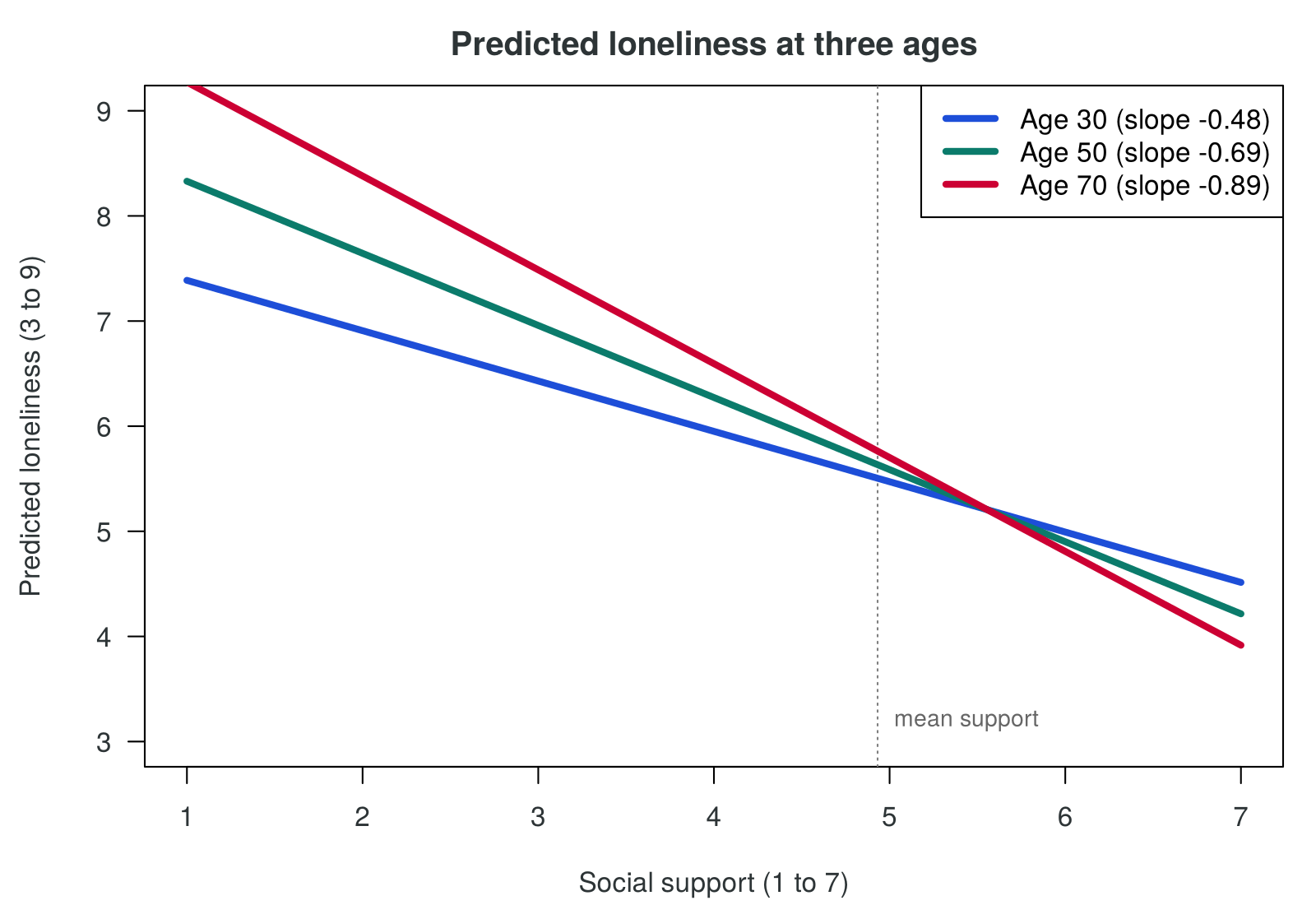
round(slopes, 3)The simple slopes of support are −0.479 at age 30, −0.686 at age 50 and −0.893 at age 70. Each 20 years of age adds about 20 × (−0.0103) = −0.21 to the slope.
R Reflect on what you just ran
Use the questions below to interpret the output you produced. Look at your console output before answering.
1. Compare the support coefficient in the uncentred model with the support_c coefficient in the centred model. Why are they so different?
age_c is the mean age of 39.5 years, so −0.58 is the support slope for a person of average age, which is a meaningful number.2. The interaction coefficient and its t value are the same in both models. Explain why centring did not change them.
3. Using the printed simple slopes, describe how the association between support and loneliness changes from age 30 to age 70, in one or two sentences suitable for a manuscript.
Table 8.5 places the coefficients of the two models side by side and gives the meaning of each one in the centred model.
Table 8.5. Coefficients of the uncentred and centred interaction models of loneliness on support and age, from Activity 8.3.
| Coefficient | Uncentred model | Centred model | Meaning in the centred model |
|---|---|---|---|
| Intercept | 6.1418 | 5.5660 | Predicted loneliness at the mean age and mean support |
| Support | −0.1685 | −0.5776 | Support slope at the mean age of 39.5 years |
| Age | 0.0575 | 0.0065 | Age slope (per year) at the mean support score of 4.93 |
| Support × age | −0.0103 (t = −7.00) | −0.0103 (t = −7.00) | Change in the support slope for each additional year of age |
The interaction coefficient and its t value are identical in the two models. Centring changes the zero point of each variable, and therefore what the main effects describe, but it leaves the interaction, the fitted values and the overall fit of the model unchanged. Centring also lowers the correlation between a main effect and its product term, but the support slope at any given age has the same estimate and standard error in both models, and the test of the interaction is unchanged.
Simple slopes for a continuous moderator
With a continuous moderator there is a different support slope at every age. The simple slope at a chosen age comes straight from the centred coefficients.
Equation 8.3 gives the simple slope at any age A, using the coefficients of the centred model in Table 8.5.
Interactive 8.2 applies Equation 8.3 to any age between 20 and 80. Moving the slider shows how the slope of support becomes steeper with age.
Figure 8.5 draws the predicted lines at ages 30, 50 and 70, the three ages whose simple slopes Activity 8.3 prints.
Simple slopes should be computed at values of the moderator that are well represented in the data. Common choices are the mean and one standard deviation above and below it, or meaningful values such as ages 30, 50 and 70. A plot with one line per chosen value is usually the clearest way to present a moderation result.
The interactions so far compare slopes of a continuous outcome, which are differences. The next part sets this additive scale beside the multiplicative scale of a logistic regression.
Additive and Multiplicative Scales
Whether an interaction exists depends on the scale on which the association is measured. In a linear regression of a continuous outcome, the interaction compares slopes, which are differences, so it is an interaction on the additive scale. In a logistic regression, the interaction term compares odds ratios, so it is an interaction on the multiplicative scale. The same data can show an interaction on one scale and none on the other, as the hypothetical example in Table 8.6 shows.
Table 8.6. A hypothetical exposure with the same risk ratio in two groups and different risk differences.
| Group | Risk without exposure | Risk with exposure | Risk difference | Risk ratio |
|---|---|---|---|---|
| Group A | 10% | 20% | 10 percentage points | 2.0 |
| Group B | 20% | 40% | 20 percentage points | 2.0 |
The risk ratio is 2.0 in both groups, so there is no interaction on the multiplicative scale. The risk difference is twice as large in group B, so there is an interaction on the additive scale. For public health decisions the additive scale is often the more relevant one, because it shows in which group an intervention would prevent more cases. For binary outcomes, reports should present the association within each group and state which scale any interaction refers to (Knol and VanderWeele, 2012; VanderWeele and Knol, 2014). The outcomes in this lesson are continuous scores, so every interaction here is on the additive scale.
The remaining step is to report the CSCS moderation result, which the last part of the section describes.
Reporting a Moderation Result
A moderation result is reported with the interaction coefficient and its confidence interval or p-value, the simple slopes, and a plot with one line per group or per chosen value of the moderator. The language describes associations. A suitable sentence for the CSCS result is: "The association between social support and loneliness differed by age group (interaction coefficient −0.31, p < 0.001). Each additional point of support was associated with a loneliness score 0.50 points lower among adults under 50 and 0.81 points lower among adults aged 50 and over." Refitting the model with "50 and over" as the reference group gives that group's slope with its own confidence interval, which can be added to the report.
The narrated walkthrough in the red card below offers a second route through the steps of Activity 8.2.
Narrated R walkthrough: Mediation and Moderation
The Mediation and Moderation walkthrough runs the moderation code in this section line by line with narration, including the age groups, the anova() comparison, the simple slopes and the plot with one line per group. Its first half covers the mediation analysis in Section 3.
This section has shown that the association between social support and loneliness is stronger at older ages, whether age is split at 50 or treated as a continuous moderator, and it has set out how such a result is reported on a stated scale. Section 3 turns to the first question of the running case, whether loneliness carries part of the association between support and depressive symptoms. The knowledge check that follows covers the material of this section.
1. Which research question is a moderation question?
2. In lm(loneliness ~ support * age_group), the coefficient support:age_group50 and over is −0.31. What does it describe?
3. In the same model, what does the support coefficient of −0.50 describe?
4. Age and support are centred at their means before fitting support * age. Which part of the output changes?
5. In group A, risk rises from 10% to 20% with exposure; in group B, it rises from 20% to 40%. Which statement is correct?
✎ Reflection
A study of 1,800 adults fits a linear regression of depressive symptoms (the PHQ-9 score, 0 to 27) on hours of physical activity per week (0 to 15), an indicator for women (1 = woman, 0 = man) and their interaction. The fitted model is: PHQ-9 = 8.20 − 0.30 × hours + 1.10 × woman − 0.20 × (hours × woman), and the interaction has p = 0.004. The mean activity in the sample is 4.0 hours per week. In this lesson, the interaction coefficient is the difference between the slopes of the two groups, the main effect of a variable describes its slope or difference when the other variable in the interaction equals zero, and centring subtracts a chosen value (usually the mean) so that zero means average. (a) Give the slope of activity for men and for women. (b) Explain what the coefficient 1.10 for women means, and calculate the difference between women and men at the mean activity of 4.0 hours. (c) Explain what would change, and what would stay the same, if hours were centred at 4.0 before fitting the model. (d) Write one sentence reporting the moderation result without causal language.
Mediation: Direct and Indirect Effects
Proportion mediated and the sensitivity parameter
Introduction
Section 1 defined the total, direct and indirect effects and the conditions under which an indirect effect can be read causally. This section estimates them for the program's first question: is social support associated with fewer depressive symptoms partly because people with more support are less lonely? The analysis follows the history of the method. It first estimates each path with an ordinary linear regression, as students did in Lesson 3, then explains why the classic four-step approach to testing mediation has been replaced, and finally estimates the indirect effect with a bootstrap confidence interval and a sensitivity analysis using the mediation package (Tingley et al., 2014).
Learning Objectives
- Fit the three regressions that give paths a, b, c and c′, and interpret each path.
- Estimate an indirect effect by the product-of-coefficients and difference methods, and explain when the two agree.
- Explain the limits of the Baron and Kenny causal steps as a test of mediation.
- Estimate the indirect, direct and total effects with bootstrap confidence intervals using
mediate(), and interpret the proportion mediated with caution. - Run and interpret a sensitivity analysis for unmeasured mediator-outcome confounding.
The section builds on the preview of mediation in Lesson 1. Box 8.6 recalls that example and its output, and it poses a retrieval question about the quantity that mediate() reports.
Box 8.6: Recall: Lesson 1, Section 1 (From DAG to Regression: A Mediation Example)
Lesson 1, Section 1 previewed mediation with simulated data in which education raises income and income improves health, with a direct path from education to health. It ran the three Baron and Kenny regressions and then the mediate() function, which reported an average causal mediation effect (ACME) of 0.30 (95% CI 0.24 to 0.35) and an average direct effect (ADE) of 0.35. That preview assumed the regression and counterfactual reasoning behind these numbers, and this section supplies it: each path comes from a linear regression of the kind fitted in Lesson 3, and the ACME and ADE rest on the counterfactual definitions given in Section 1.
Retrieval question. What does the ACME reported by mediate() estimate?
The first step is to estimate the paths of the mediation diagram with three regressions, which the next part does.
Three Regressions, Four Paths
With support as the exposure (X), loneliness as the mediator (M) and depressive symptoms as the outcome (Y), three linear regressions give every path in the mediation diagram. The outcome model includes both the exposure and the mediator, so that path b describes the association between loneliness and depressive symptoms among people with the same level of support.
Table 8.7 lists the three models, the R code for each, the coefficient that is used from it and the path that the coefficient estimates.
Table 8.7. The three regressions of a simple mediation analysis and the paths they estimate.
| Model | R code | Coefficient used | Path |
|---|---|---|---|
| Total-effect model | lm(depression ~ support) | support | c (total effect) |
| Mediator model | lm(loneliness ~ support) | support | a |
| Outcome model | lm(depression ~ support + loneliness) | loneliness and support | b and c′ (direct effect) |
The models in this lesson have no covariates, so that the numbers match the narrated walkthrough. In a manuscript, the confounders identified in the DAG (for example age, gender and income) would be added to the mediator model and to the outcome model, so that paths a and b are adjusted for the common causes of the exposure and mediator and of the mediator and outcome.
Activity 8.4 fits the three models to the CSCS data and computes the indirect effect by both of the methods described in the next part.
This activity fits the three regressions and calculates the indirect effect in two ways. Each model is printed as its coefficients with 95% confidence intervals, using cbind(estimate = coef(model), confint(model)) as in Lesson 4.
github_url <- "https://raw.githubusercontent.com/jorgeandr3s/heal/main/cscs/public_data/CSCS2025_full_cleaned_deidentified_data_and_metadata.RData"
load(url(github_url))                                 # creates a data frame called data
data <- data[data$SURVEY_collection_year == 2021, ]   # keep the 2021 wave
med_data <- data.frame(
  support    = data$PSYCH_zimet_multidimensional_social_support_scale_score,
  loneliness = data$LONELY_ucla_loneliness_scale_score,
  depression = data$WELLNESS_phq_score,
  age        = data$DEMO_age)
med_data <- na.omit(med_data)   # the same people in every model
nrow(med_data)# Path c, the total effect: support -> depression
model_total <- lm(depression ~ support, data = med_data)
round(cbind(estimate = coef(model_total), confint(model_total)), 3) # with 95% CIsPath c, the total effect: each point of support is associated with a PHQ-2 score 0.560 points lower (95% CI −0.608 to −0.511).
# Path a: support -> loneliness
model_a <- lm(loneliness ~ support, data = med_data)
round(cbind(estimate = coef(model_a), confint(model_a)), 3) # with 95% CIsPath a: each point of support is associated with a loneliness score 0.626 points lower (95% CI −0.676 to −0.576).
# Path b (loneliness -> depression) and path c' (the direct effect)
model_b <- lm(depression ~ support + loneliness, data = med_data)
round(cbind(estimate = coef(model_b), confint(model_b)), 3) # with 95% CIsThe outcome model gives two paths. Path b: among people with the same support score, each point of loneliness is associated with a PHQ-2 score 0.366 points higher (95% CI 0.334 to 0.397). Path c′, the direct effect: among people with the same loneliness score, each point of support is associated with a PHQ-2 score 0.331 points lower (95% CI −0.380 to −0.282). The direct effect is smaller than the total effect of −0.560, because part of the total runs through loneliness.
a <- coef(model_a)["support"]
b <- coef(model_b)["loneliness"]
c_total  <- coef(model_total)["support"]
c_direct <- coef(model_b)["support"]
a * b                  # indirect effect: product of coefficients
c_total - c_direct # indirect effect: difference methodBoth methods give an indirect effect of −0.2289. R labels both results support because the first number in each calculation was taken from the support coefficient.
R Reflect on what you just ran
Use the questions below to interpret the output you produced. Look at your console output before answering.
1. Report paths a, b, c and c′ with their 95% confidence intervals, and say which model each comes from.
lm(depression ~ support)) is −0.560 (−0.608 to −0.511). Path a (from lm(loneliness ~ support)) is −0.626 (−0.676 to −0.576). Path b, the loneliness coefficient in lm(depression ~ support + loneliness), is 0.366 (0.334 to 0.397), and path c′, the support coefficient in the same model, is −0.331 (−0.380 to −0.282).2. Show that the product-of-coefficients and difference methods give the same indirect effect, and explain why they agree here.
3. What share of the total association does the indirect effect represent? Write one sentence reporting it in language suited to cross-sectional data.
Figure 8.6 places the estimates from Activity 8.4 on the mediation diagram of Figure 8.2.
The three regressions give every path, and the indirect effect follows from them. The next part sets out the two ways of calculating it.
Product-of-Coefficients and Difference Methods
The indirect effect can be calculated in two ways. The product-of-coefficients method multiplies path a by path b. The difference method subtracts the direct effect from the total effect.
Equation 8.4 applies both methods to the CSCS estimates from Activity 8.4.
The product-of-coefficients method has an intuitive reading. A support score one point higher goes with a loneliness score 0.626 points lower (path a), and each point of loneliness goes with 0.366 more PHQ-2 points among people with the same support (path b), so the pathway through loneliness corresponds to 0.626 × 0.366 = 0.229 fewer PHQ-2 points. The two methods agree exactly only when the mediator and outcome models are linear regressions fitted to the same people. When the outcome is binary and modelled with logistic regression, c − c′ and a × b can differ, because odds ratios change when a variable is added to the model even without confounding. The counterfactual approach used by mediate() handles such models consistently (Imai, Keele and Tingley, 2010; VanderWeele, 2015).
Figure 8.7 shows the result of the decomposition as two bars, with the total association above and its direct and indirect parts below.
The product a × b is the quantity of interest in a mediation analysis. The older causal steps, which the next part describes, never test this product.
The Baron and Kenny Causal Steps
For about two decades, most published mediation analyses followed the causal steps of Baron and Kenny (1986). Mediation was claimed when four conditions were met: the exposure predicted the outcome (path c), the exposure predicted the mediator (path a), the mediator predicted the outcome with the exposure held constant (path b), and the exposure coefficient shrank when the mediator was added (c′ smaller than c). If c′ fell to zero, the result was called full mediation, and otherwise partial mediation. The steps are still described in many textbooks, and students will meet them in published papers. Students who took HSCI 341 met these steps in Lesson 1, Section 2 of that course. Methodologists no longer recommend them as a test of mediation, for the reasons below (MacKinnon et al., 2002; Hayes, 2009; Zhao, Lynch and Chen, 2010).
The accordion below gives these reasons, one in each of its five panels.
The quantity of interest is a × b, yet the steps test a and b separately and never test their product or give it a confidence interval. Separate significance tests are a poor guide to whether the product differs from zero.
Requiring every step to be statistically significant makes the approach less powerful than a direct test of the indirect effect, so real indirect effects are often missed in samples of ordinary size (Fritz and MacKinnon, 2007).
The first step requires a significant total effect. When the direct and indirect effects have opposite signs, they can cancel out, so that the total effect is close to zero even though a real indirect effect exists. This pattern is called inconsistent mediation, or suppression, and the first step would stop the analysis before it was found.
Whether c′ is "significantly different from zero" depends largely on the sample size. In the CSCS, with 3,110 people, almost any direct effect is significant, so the result would nearly always be called partial mediation, while the same estimates in a sample of 100 people could be called full mediation. The labels describe statistical power more than they describe the pathway, so current guidance reports the size of the direct and indirect effects with confidence intervals instead (Rucker et al., 2011).
The steps use the word "causal", yet they say nothing about temporal order or confounding of the mediator and the outcome, which Section 1 showed are needed for a causal reading.
An early direct test of a × b, the Sobel test, divides the product by an approximate standard error and compares the result with a normal distribution. The sampling distribution of a product of two estimates is usually skewed, so a symmetric normal interval can be misleading. The bootstrap avoids this assumption (Preacher and Hayes, 2008). It draws many new samples of the same size from the data with replacement, refits the models in each one, and takes the 2.5th and 97.5th percentiles of the resulting indirect effects as the 95% confidence interval.
The next part estimates the indirect effect for the running case with a bootstrap confidence interval, using the mediate() function.
Estimating the Indirect Effect with mediate()
The mediate() function in the mediation package takes the mediator model and the outcome model, names the exposure (treat) and the mediator, and returns four quantities. Their names come from the counterfactual definitions in Section 1, which is why the word "causal" appears in them.
The four cards below define the four quantities and give the path, or combination of paths, to which each corresponds in a linear model.
Activity 8.5 estimates the four quantities for the running case with 1,000 bootstrap samples and then runs the sensitivity analysis described in Box 8.4.
This activity uses the mediation package. Install it once with install.packages("mediation") if it is not yet installed. The bootstrap refits the two models 1,000 times, so mediate() takes about 15 seconds on a laptop, and medsens() takes a few seconds more. set.seed(2021) makes the random resampling repeatable, so your numbers will match the ones below.
# install.packages("mediation")   # run once, if not yet installed
library(mediation)
github_url <- "https://raw.githubusercontent.com/jorgeandr3s/heal/main/cscs/public_data/CSCS2025_full_cleaned_deidentified_data_and_metadata.RData"
load(url(github_url))                                 # creates a data frame called data
data <- data[data$SURVEY_collection_year == 2021, ]   # keep the 2021 wave
med_data <- data.frame(
  support    = data$PSYCH_zimet_multidimensional_social_support_scale_score,
  loneliness = data$LONELY_ucla_loneliness_scale_score,
  depression = data$WELLNESS_phq_score,
  age        = data$DEMO_age)
med_data <- na.omit(med_data)   # the same people in every model
model_a <- lm(loneliness ~ support, data = med_data)                # path a
model_b <- lm(depression ~ support + loneliness, data = med_data)   # paths b and c-prime
This chunk loads the package and the data and fits the mediator model (path a) and the outcome model (paths b and c′). It prints only messages from the package.
set.seed(2021)   # makes the bootstrap results repeatable
med_result <- mediate(model_a, model_b,
                      treat = "support", mediator = "loneliness",
                      boot = TRUE, sims = 1000)
summary(med_result)Reading the output. The ACME row is the indirect effect, −0.229 (95% CI −0.256 to −0.201), which matches a × b from Activity 8.4. The ADE row is the direct effect, −0.331 (95% CI −0.386 to −0.279), and the Total Effect row is −0.560 (95% CI −0.618 to −0.509). Prop. Mediated is 0.41 (95% CI 0.36 to 0.46). The intervals come from the 1,000 bootstrap samples (the percentile method). The p-values are printed as below 2.2 × 10⁻¹⁶, the smallest value R displays; bootstrap p-values are approximate, and the intervals carry the main information.
plot(med_result, xlim = c(-0.7, 0)) # the three effects with 95% CIsThis line draws the plot of the three effects shown in Figure 8.8.
# Sensitivity analysis: how strong would unmeasured confounding of
# loneliness and depression have to be to remove the indirect effect?
sens <- medsens(med_result, rho.by = 0.1, effect.type = "indirect", sims = 100)
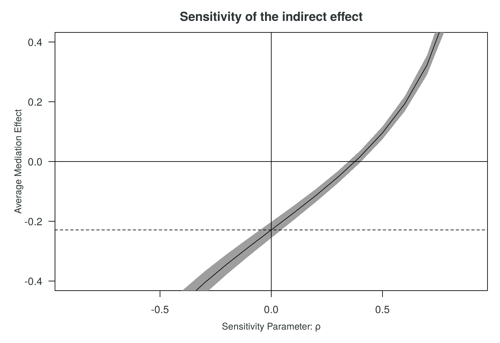
summary(sens)Reading the output. Rho at which ACME = 0: 0.4 means that the indirect effect would fall to zero if the residuals of the loneliness model and the depression model were correlated at about 0.4 because of an unmeasured confounder. The Sensitivity Region table lists the values of ρ at which the confidence interval for the ACME includes zero; with steps of 0.1, only ρ = 0.4 does. The line R^2_M*R^2_Y* at which ACME = 0: 0.16 gives the same threshold as the product of the shares of remaining variance in loneliness and in depressive symptoms that the confounder would need to explain (for example 0.4 × 0.4). With rho.by = 0.1 the threshold is located to the nearest 0.1.
R Reflect on what you just ran
Use the questions below to interpret the output you produced. Look at your console output and plots before answering.
1. Report the ACME with its 95% confidence interval, and interpret it in one sentence that is suitable for cross-sectional data.
2. The proportion mediated is 0.41 (95% CI 0.36 to 0.46). Explain what it means and give two reasons why proportions mediated must be interpreted with caution in general.
3. The sensitivity analysis reports that the ACME equals zero at ρ = 0.4. Explain what this means in plain language and name one unmeasured variable that could produce such confounding.
Figure 8.8 shows the plot drawn in Activity 8.5, in which the indirect, direct and total effects each appear with a 95% bootstrap confidence interval.
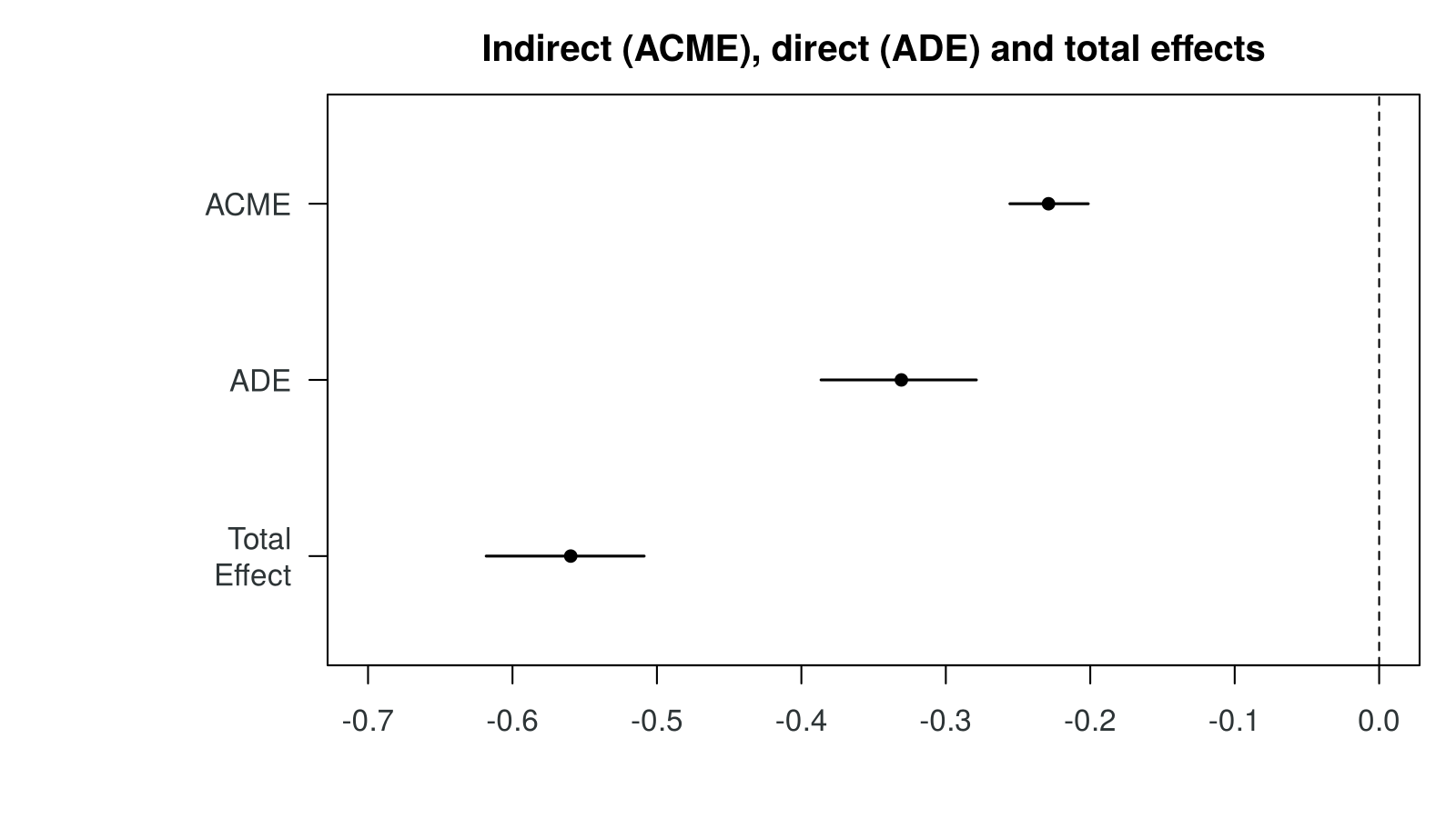
plot(med_result): the indirect effect (ACME), the direct effect (ADE) and the total effect, each with its 95% bootstrap confidence interval. All three intervals lie well to the left of zero.The proportion mediated, read with caution
The proportion mediated is 0.41 (95% CI 0.36 to 0.46): loneliness statistically accounts for about 41% of the association between support and depressive symptoms. The figure is easy to communicate, and it is also easy to misuse. Because it is a ratio of two estimates, it becomes unstable when the total effect is small, and its interval can then be very wide. When the direct and indirect effects have opposite signs, it can exceed 1 or fall below 0, values that have no sensible reading as a share. In the CSCS the total effect is large and precisely estimated and both parts have the same sign, so the proportion is stable. It still describes how an association divides in these data, and it does not say that 41% of any benefit of support on mental health works through loneliness.
The estimates from mediate() rest on the assumption of no unmeasured mediator-outcome confounding. The next part examines how far the conclusion depends on that assumption.
Sensitivity Analysis for Unmeasured Mediator-Outcome Confounding
Section 1 showed that a causal reading of the indirect effect requires no unmeasured confounding of the mediator and the outcome, a condition that cannot be checked from the data. A history of depression, for example, could make a person both lonelier and more likely to report depressive symptoms now. The medsens() function asks how strong such confounding would need to be to change the conclusion (Imai, Keele and Tingley, 2010). Unmeasured confounding of loneliness and depressive symptoms would make the residuals of the mediator model and of the outcome model correlated. The sensitivity parameter ρ (rho) is that correlation. The analysis assumes ρ = 0, and medsens() recalculates the indirect effect for a range of other values.
Figure 8.9 plots the indirect effect that medsens() recalculates across values of ρ, together with its confidence band.
The indirect effect falls to zero when ρ is about 0.4. An equivalent reading uses the second line of the summary: an unmeasured confounder would need to explain about 40% of the remaining variance in both loneliness and depressive symptoms (0.4 × 0.4 = 0.16) to remove the indirect effect. That is a strong confounder, but a variable such as a history of depression could plausibly be one, so the result shows that the indirect association is reasonably resistant to this kind of confounding without ruling it out. The sensitivity analysis addresses only mediator-outcome confounding. It says nothing about the order of the variables in time, which remains the main limitation of the CSCS data.
With the estimates and their sensitivity to confounding in hand, the remaining task is to report the analysis, which the last part of the section describes.
Reporting a Mediation Analysis
The AGReMA statement (Lee et al., 2021) gives a checklist for reporting mediation analyses of trials and observational studies. Its main elements can be embedded in a few sentences: the assumed causal structure (a DAG), the timing of each measurement, the covariates in the mediator and outcome models, the estimation method and number of bootstrap samples, the indirect, direct and total effects with confidence intervals, a sensitivity analysis, and the limitations of the design.
Box 8.7 shows how several of these elements read in a results paragraph for the CSCS analysis.
"We examined whether loneliness statistically accounted for part of the association between perceived social support and depressive symptoms among 3,110 participants in the 2021 wave of the Canadian Social Connection Survey. Indirect, direct and total associations were estimated with linear mediator and outcome models and the mediation package in R, with 95% confidence intervals from 1,000 nonparametric bootstrap samples. Each additional point of support was associated with a PHQ-2 score 0.56 points lower (95% CI −0.62 to −0.51). The indirect association through loneliness was −0.23 (95% CI −0.26 to −0.20) and the direct association was −0.33 (95% CI −0.39 to −0.28), so loneliness statistically accounted for about 41% of the total association (95% CI 36% to 46%). A sensitivity analysis indicated that the indirect association would be removed by unmeasured confounding of loneliness and depressive symptoms that induced a residual correlation of about 0.4. Because all measures were collected at the same time, these results describe a pattern of associations consistent with a pathway through loneliness and do not establish its direction."
The narrated walkthrough in the red card below offers a second route through the regressions of Activity 8.4 and the mediate() analysis of Activity 8.5.
Narrated R walkthrough: Mediation and Moderation
The first half of the Mediation and Moderation walkthrough runs the three regressions, the a × b calculation and the mediate() analysis of this section line by line, with narration and diagrams of each path.
This section has estimated the indirect association of social support with depressive symptoms through loneliness, −0.23 PHQ-2 points per point of support or about 41% of the total, and it has shown that this association would fall to zero if mediator-outcome confounding produced a residual correlation of about 0.4. Section 4 writes the same model as a path model and extends it to a second outcome. The knowledge check that follows covers the material of this section.
1. In the CSCS data, path a (support to loneliness) is −0.626 and path b (loneliness to depressive symptoms, holding support constant) is 0.366. What is the indirect effect by the product-of-coefficients method?
2. Which is a reason the Baron and Kenny causal steps are no longer recommended as a test of mediation?
3. The mediate() output gives ACME = −0.229 (95% CI −0.256 to −0.201) for the cross-sectional CSCS data. Which interpretation is most appropriate?
4. Why is the bootstrap preferred to a normal-theory test (such as the Sobel test) for the confidence interval of an indirect effect?
5. A sensitivity analysis finds that the ACME equals zero when ρ = 0.4. What does this mean?
✎ Reflection
A cohort study of 2,400 adults measures neighbourhood walkability at baseline (exposure, a score from 0 to 100), weekly minutes of physical activity one year later (mediator), and systolic blood pressure two years after baseline (outcome, mmHg). Both the mediator model and the outcome model are adjusted for age, gender and income. The mediate() output, with 1,000 bootstrap samples and the walkability score expressed per 10 points, is: ACME −0.40 (95% CI −0.62 to −0.21); ADE −0.35 (95% CI −0.90 to 0.18); Total Effect −0.75 (95% CI −1.31 to −0.22); Prop. Mediated 0.53 (95% CI 0.25 to 1.62). A sensitivity analysis gives ρ at which ACME = 0 of 0.15. In this lesson, the ACME is the indirect effect, the ADE is the direct effect, the proportion mediated is the ACME divided by the total effect, and ρ is the correlation between the residuals of the mediator and outcome models that unmeasured mediator-outcome confounding would induce. (a) Interpret the ACME and the ADE. (b) Explain why the confidence interval for the proportion mediated is so wide and why a label of "full mediation" would be unwise. (c) Explain what the sensitivity result means. (d) This study has temporal order, unlike the CSCS. State whether you would use causal language and why.
Path Analysis and the Road to Structural Equation Modelling
Introduction
Sections 2 and 3 fitted one regression at a time. A path model writes all of the regressions in an analysis as one diagram and estimates them together. This has three advantages. Several outcomes and several pathways can be handled at once, the indirect effects can be defined and tested inside the model, and a whole model can be compared with a simpler one that leaves some paths out. This section expresses the mediation model from Section 3 as a path diagram, fits it with the lavaan package (Rosseel, 2012), extends it to two outcomes, compares two versions, and reports the chosen model. It closes by adding a latent variable, which turns the path model into a structural equation model (SEM) and connects this lesson to the confirmatory factor analysis in Lesson 7.
Learning Objectives
- Draw and read a path diagram using the conventions for observed variables, latent variables, paths and covariances.
- Specify a path model in lavaan syntax with labelled paths and a defined indirect effect.
- Fit full and partial mediation models with two outcomes and compare them with a chi-square difference test and the AIC.
- Report a path model with bootstrap confidence intervals, standardized coefficients, R-squared values and a figure.
- Explain how adding a measurement model with latent variables extends path analysis to structural equation modelling.
The section starts with the symbols of a path diagram and the lavaan syntax that turns a diagram into a model.
Path Diagrams
Path analysis was introduced by the geneticist Sewall Wright (1921) as a way of tracing correlations through chains of causes. A path diagram uses a small set of symbols, and the same symbols are used in SEM.
Table 8.8 lists the symbols with their meaning and an example of each from this section.
Table 8.8. The symbols of a path diagram.
| Symbol | Meaning | Example in this section |
|---|---|---|
| Rectangle | An observed variable, recorded in the dataset | The loneliness score, the PHQ-2 score |
| Oval | A latent variable, measured indirectly through several observed items | A loneliness factor measured by three UCLA items |
| Single-headed arrow | A regression path from a predictor to an outcome | Support → loneliness |
| Double-headed arrow | A covariance (or correlation) with no direction assumed | The residuals of depression and anxiety |
| Residual (often a small circle or an unlabelled arrow) | The part of an endogenous variable that the model does not explain | Everything else that affects loneliness |
A variable with no arrows pointing at it is exogenous: its causes lie outside the model, and in this section support is the only exogenous variable. A variable with at least one arrow pointing at it is endogenous, and the model has an equation for it. Loneliness, depressive symptoms and anxiety symptoms are endogenous. Each single-headed arrow in the diagram is a coefficient in one of those equations, so a path model with three endogenous variables is a set of three regressions fitted together.
To estimate these regressions together, the diagram has to be written as a model that R can fit, which is the subject of the next part.
Writing a Path Model in lavaan
The lavaan package describes a model as a block of text inside single quotes, with one equation or relationship on each line. Four operators cover everything in this lesson.
Table 8.9 sets out the four operators, how each is read, an example of each and the element of the path diagram that each one produces.
Table 8.9. The four lavaan operators used in this lesson.
| Operator | Read as | Example | In the diagram |
|---|---|---|---|
~ | is regressed on | loneliness ~ support | Arrow from support to loneliness |
~~ | covaries with | depression ~~ anxiety | Double-headed arrow |
=~ | is measured by | Lonely =~ companionship + left_out + isolated | Oval with arrows to its items |
:= | is defined as | indirect := a * b | A quantity computed from labelled paths |
A label is written in front of a predictor with an asterisk, as in loneliness ~ a * support, which names the path from support to loneliness a. Labels make it possible to define the indirect effect (a * b) and the total effect (c + a * b) inside the model, and lavaan then reports their estimates and standard errors with the other parameters. The model is fitted with sem(model, data = ...).
The simple mediation model in lavaan
The first activity rebuilds the mediation model from Section 3 in lavaan. The path model uses people with complete data on four variables (support, loneliness, depressive symptoms and anxiety symptoms), because the second activity adds anxiety as a second outcome. This leaves 3,099 people, eleven fewer than in Sections 2 and 3, so the estimates differ slightly in the third decimal place.
Activity 8.6 fits the model and defines the indirect and total effects from its labelled paths.
This activity uses the lavaan package. Install it once with install.packages("lavaan") if it is not yet installed. The data frame path_data adds anxiety symptoms to the variables used so far and keeps the people who answered all four questions.
# install.packages("lavaan")   # run once, if not yet installed
library(lavaan)
github_url <- "https://raw.githubusercontent.com/jorgeandr3s/heal/main/cscs/public_data/CSCS2025_full_cleaned_deidentified_data_and_metadata.RData"
load(url(github_url))                                 # creates a data frame called data
data <- data[data$SURVEY_collection_year == 2021, ]   # keep the 2021 wave
path_data <- data.frame(
  support    = data$PSYCH_zimet_multidimensional_social_support_scale_score,
  loneliness = data$LONELY_ucla_loneliness_scale_score,
  depression = data$WELLNESS_phq_score,
  anxiety    = data$WELLNESS_gad_score)   # GAD-2 anxiety symptoms, 0 to 6
path_data <- na.omit(path_data)          # people with all four variables
nrow(path_data)The path models use 3,099 people with complete data on support, loneliness, depressive symptoms and anxiety symptoms.
model_med <- '
  loneliness ~ a * support
  depression ~ b * loneliness + c * support
  indirect := a * b
  total    := c + a * b
'
fit_med <- sem(model_med, data = path_data)
summary(fit_med)Reading the output. Under Regressions, the labelled paths are a = −0.627, b = 0.365 and c = −0.329, which match the linear regressions of Section 3 (−0.626, 0.366 and −0.331) apart from the eleven people who are now excluded. In lavaan the label c names the direct path, which Section 3 called c′. Under Defined Parameters, the indirect effect is −0.229 (standard error 0.014) and the total effect is −0.559. Under Variances, the dots before .loneliness and .depression mark residual variances. Degrees of freedom 0 and a test statistic of 0.000 show that the model is saturated.
R Reflect on what you just ran
Use the questions below to interpret the output you produced. Look at your console output before answering.
1. Compare paths a, b and c in the lavaan output with the paths from the linear regressions in Section 3 (a = −0.626, b = 0.366, c′ = −0.331). Why are they very close but not identical?
lm(). They differ slightly in the third decimal place because path_data drops the eleven people who are missing the anxiety score, so the path model uses 3,099 people instead of 3,110.2. Report the indirect and total effects from the Defined Parameters section, and explain how lavaan calculated them.
indirect := a * b and total := c + a * b, and it estimated their standard errors from the standard errors and covariances of the paths. These normal-theory standard errors are replaced by bootstrap intervals in the next activity.3. The output shows 0 degrees of freedom and a test statistic of 0.000. What does this mean for testing the fit of this model?
The simple mediation model has zero degrees of freedom. It estimates five parameters (three paths and two residual variances), and the data supply exactly five pieces of information about the relationships among the three variables, once the variance of support is set aside. A model like this is called saturated or just-identified. It reproduces the observed covariances exactly, so its chi-square is 0 and its fit cannot be tested. Fit becomes testable only when a model leaves some paths out, which is what the two-outcome models do.
A Path Model with Two Outcomes
The CSCS also includes the two-item Generalized Anxiety Disorder scale (GAD-2; Kroenke et al., 2007), scored from 0 to 6. The analyst asks whether loneliness links support to both depressive and anxiety symptoms, and compares two models.
Figure 8.10 draws the two models in one diagram, with the direct paths that only Model 2 contains shown as dashed arrows.
Model 1 contains no direct paths from support to the outcomes. It corresponds to what the Baron and Kenny tradition calls full mediation. Model 2 adds the direct paths and labels every path so that the two indirect effects can be defined. Both models include depression ~~ anxiety, which allows the parts of depressive and anxiety symptoms that loneliness and support leave unexplained to be correlated. Leaving this line out would assume that nothing else links the two outcomes, which is implausible for two measures of distress.
Activity 8.7 fits both models, compares them and reports the chosen model with bootstrap confidence intervals, standardized coefficients and R-squared values.
This activity continues from the previous one in the same R session, using path_data. It fits the two models in Figure 8.10, compares them, and reports the chosen model. The bootstrap step refits the model 1,000 times and takes about a minute. R may print a warning that a few bootstrap runs failed or did not converge. With 1,000 runs, losing a handful does not change the intervals in any meaningful way.
# Model 1, full mediation: no direct paths from support
model_full <- '
  loneliness ~ support
  depression ~ loneliness
  anxiety    ~ loneliness
  depression ~~ anxiety
'
fit_full <- sem(model_full, data = path_data)
fitMeasures(fit_full, c("chisq", "df", "pvalue", "cfi", "tli", "rmsea", "srmr"))Model 1 has 2 degrees of freedom, one for each direct path it leaves out. Its chi-square is 173.8 (p printed as 0.000), its RMSEA is 0.166, its CFI is 0.942 and its TLI is 0.827: by every index except the SRMR (0.071), the model fits poorly.
# Model 2, partial mediation: adds a direct path to each outcome
model_partial <- '
  loneliness ~ a * support
  depression ~ b1 * loneliness + c1 * support
  anxiety    ~ b2 * loneliness + c2 * support
  depression ~~ anxiety
  indirect_dep := a * b1
  indirect_anx := a * b2
'
fit_partial <- sem(model_partial, data = path_data)
fitMeasures(fit_partial, c("chisq", "df", "cfi", "rmsea", "srmr"))Model 2 has 0 degrees of freedom, so it is saturated and fits perfectly by construction.
anova(fit_full, fit_partial) # chi-square difference test, AIC and BICReading the output. The chi-square difference is 173.76 on 2 degrees of freedom (p < 2.2 × 10⁻¹⁶), so removing the two direct paths makes the fit much worse. The AIC is 32,864 for Model 2 and 33,033 for Model 1, and the BIC is 32,918 and 33,076; lower values are better, so both favour Model 2. The RMSEA column (0.166) describes the misfit added by the constraint.
set.seed(2021)
fit_boot <- sem(model_partial, data = path_data,
                se = "bootstrap", bootstrap = 1000)
est <- parameterEstimates(fit_boot, boot.ci.type = "perc")
est[est$op %in% c("~", ":="), c("lhs", "op", "rhs", "est", "ci.lower", "ci.upper")]The table keeps the regression paths (~) and the defined indirect effects (:=). The columns ci.lower and ci.upper are 95% percentile bootstrap intervals. The indirect association for depressive symptoms is −0.229 (−0.257 to −0.203), and for anxiety symptoms it is −0.217 (−0.246 to −0.191).
std <- standardizedSolution(fit_boot)
std[std$lhs != std$rhs, c("lhs", "op", "rhs", "est.std")]   # paths, covariance, indirect
lavInspect(fit_boot, "rsquare") # variance explained in each outcomeThe est.std column gives standardized estimates: −0.403 for support to loneliness, 0.381 and 0.371 for loneliness to the two outcomes, and −0.221 and −0.150 for the direct paths. The ~~ row is the residual correlation of the outcomes (0.472), and the standardized indirect effects are −0.154 and −0.149. The R-squared values are 0.162 for loneliness, 0.262 for depressive symptoms and 0.204 for anxiety symptoms.
R Reflect on what you just ran
Use the questions below to interpret the output you produced. Look at your console output before answering.
1. Using the output of fitMeasures(fit_full, ...), explain whether Model 1 fits the data, with reference to at least three indices and their usual guides.
2. Which model do the chi-square difference test and the AIC favour? Explain the reasoning in two or three sentences, and say why the result should not be summarized as "partial mediation".
3. Report the two indirect associations with their bootstrap confidence intervals and the R-squared for depressive symptoms, in one or two sentences suitable for a manuscript.
Reading the fit indices
Fit indices describe how well a model with some paths left out reproduces the observed covariances. The guides for good fit in Table 8.10 follow Hu and Bentler (1999), and the description of an RMSEA above 0.10 as poor follows Browne and Cudeck (1993). All of these guides are rules of thumb, and they work best when several indices are read together (Kline, 2016).
Table 8.10. Common fit indices, what each measures, the usual guide for good fit and the value for Model 1.
| Index | What it measures | Usual guide for good fit | Model 1 |
|---|---|---|---|
| Chi-square test | Whether the model's covariances differ from the observed ones; in large samples it rejects almost every model | p above 0.05 | 173.8 on 2 df, p < 0.001 |
| CFI (comparative fit index) | Improvement over a model in which no variables are related | 0.95 or higher | 0.942 |
| TLI (Tucker-Lewis index) | Like the CFI, with a penalty for complexity | 0.95 or higher | 0.827 |
| RMSEA (root mean square error of approximation) | Misfit per degree of freedom | 0.06 or lower; above 0.10 is poor | 0.166 |
| SRMR (standardized root mean square residual) | Average difference between observed and model correlations | 0.08 or lower | 0.071 |
Model 1 fits poorly. Its RMSEA of 0.166 is well above 0.10, its TLI is 0.827 and its CFI is just below 0.95. Only the SRMR falls inside its guide. Model 2 has 0 degrees of freedom, so it is saturated, and its perfect fit indices (CFI 1, RMSEA 0, SRMR 0) carry no information about whether it is correct.
Comparing nested models
Model 1 is nested in Model 2: fixing the two direct paths of Model 2 at zero gives Model 1. Nested models fitted to the same people can be compared with a chi-square difference test, which anova(fit_full, fit_partial) reports. The difference is 173.76 on 2 degrees of freedom (one for each path that Model 1 removes), with p < 2.2 × 10⁻¹⁶, so removing the direct paths makes the fit much worse. The Akaike information criterion (AIC), which Lesson 4 used to compare count models, agrees: it is 32,864 for Model 2 and 33,033 for Model 1, a difference of about 170 points in favour of Model 2. The BIC (32,918 and 33,076) points the same way.
In words, the data are inconsistent with a model in which support is related to depressive and anxiety symptoms only through loneliness. Section 3 explained that labels such as "full" and "partial" mediation depend mainly on sample size. With more than 3,000 people, a model with no direct paths was always likely to be rejected, so the report describes the size of each direct and indirect path with its confidence interval and does not rest on a label.
Results from the chosen model
The second activity refits Model 2 with 1,000 bootstrap samples and reports percentile confidence intervals for every path and for the two indirect effects. It then reports the standardized coefficients, which express each path in standard deviation units, so that paths measured on different scales can be compared, and the R-squared for each endogenous variable, the proportion of its variance that the model explains.
Table 8.11 collects these results from Activity 8.7 for every path and for the two indirect effects.
Table 8.11. Unstandardized estimates with 95% bootstrap confidence intervals and standardized estimates from Model 2 (n = 3,099).
| Path or quantity | Unstandardized estimate (95% bootstrap CI) | Standardized |
|---|---|---|
| Support → loneliness (a) | −0.627 (−0.677 to −0.574) | −0.403 |
| Loneliness → depression (b1) | 0.365 (0.331 to 0.402) | 0.381 |
| Support → depression, direct (c1) | −0.329 (−0.386 to −0.273) | −0.221 |
| Loneliness → anxiety (b2) | 0.346 (0.310 to 0.379) | 0.371 |
| Support → anxiety, direct (c2) | −0.217 (−0.273 to −0.160) | −0.150 |
| Indirect, depression (a × b1) | −0.229 (−0.257 to −0.203) | −0.154 |
| Indirect, anxiety (a × b2) | −0.217 (−0.246 to −0.191) | −0.149 |
| Residual correlation, depression and anxiety | (not shown) | 0.472 |
Both indirect associations are clearly different from zero. The indirect association for depressive symptoms (−0.229) matches the ACME from Section 3, and the indirect association for anxiety symptoms is similar in size (−0.217). The model explains 16% of the variance in loneliness, 26% in depressive symptoms and 20% in anxiety symptoms. The residual correlation of 0.47 shows that depressive and anxiety symptoms remain strongly related after support and loneliness are taken into account, which justifies the covariance in the model.
The comparison favours Model 2, and Table 8.11 gives its estimates. The next part shows how such a model is presented in a report.
Reporting a Path Model
A path model is usually reported with a figure that shows the standardized coefficients, a table of unstandardized estimates with confidence intervals, the fit indices of each model compared, the indirect effects with bootstrap intervals, and the software, estimator and handling of missing data. Figure 8.11 is a reporting figure for Model 2.
A matching results sentence is: "In a path model fitted to 3,099 CSCS participants, the indirect association of social support with depressive symptoms through loneliness was −0.23 (95% bootstrap CI −0.26 to −0.20), and with anxiety symptoms it was −0.22 (95% CI −0.25 to −0.19). A model without direct paths from support to the outcomes fitted poorly (RMSEA 0.17, CFI 0.94) and significantly worse than a model with them (chi-square difference 173.8 on 2 df, p < 0.001; AIC 33,033 compared with 32,864)." The sentence describes associations, as every result from these cross-sectional data must.
The last part of the section asks what changes when one of the observed scores in a path model is replaced by a latent variable.
From Path Analysis to Structural Equation Modelling
Every variable in the path models so far is an observed score, and every score contains measurement error. Lesson 7 showed that measurement error weakens (attenuates) correlations, and that a latent variable measured by several items separates the shared variation in the items from their error. A structural equation model joins the two ideas. Its measurement model is a confirmatory factor analysis, which defines each latent variable by its items with the =~ operator, and its structural model is a set of paths among the latent and observed variables, written with ~ exactly as in this section.
Figure 8.12 shows such a model for the CSCS data, with a latent loneliness factor measured by the three UCLA items in place of the observed loneliness score.
Worked code 8.1 gives the lavaan code and output for the model in Figure 8.12, and the paragraph after it compares the estimates with those of the path model.
This example fits the model in Figure 8.12. It uses the three UCLA loneliness items (each scored 1 = hardly ever, 2 = some of the time, 3 = often) in place of the total score. The same 3,110 people as in Sections 2 and 3 have complete data. The code runs on its own after library(lavaan) is installed. It is an example to read, and the knowledge check does not ask you to run it.
library(lavaan)
github_url <- "https://raw.githubusercontent.com/jorgeandr3s/heal/main/cscs/public_data/CSCS2025_full_cleaned_deidentified_data_and_metadata.RData"
load(url(github_url))                                 # creates a data frame called data
data <- data[data$SURVEY_collection_year == 2021, ]   # keep the 2021 wave
sem_data <- data.frame(
  companionship = data$LONELY_ucla_loneliness_scale_companionship_num,
  left_out      = data$LONELY_ucla_loneliness_scale_left_out_num,
  isolated      = data$LONELY_ucla_loneliness_scale_isolated_num,
  support       = data$PSYCH_zimet_multidimensional_social_support_scale_score,
  depression    = data$WELLNESS_phq_score)
sem_data <- na.omit(sem_data)
nrow(sem_data)model_sem <- '
# measurement model: a latent loneliness factor with three items
Lonely =~ companionship + left_out + isolated
# structural model: the paths between support, Lonely and depression
Lonely ~ a * support
depression ~ b * Lonely + c * support
indirect := a * b
'
fit_sem <- sem(model_sem, data = sem_data)
fitMeasures(fit_sem, c("chisq", "df", "cfi", "rmsea", "srmr"))
std <- standardizedSolution(fit_sem)
std[std$op %in% c("=~", "~", ":="), c("lhs", "op", "rhs", "est.std", "pvalue")]The model fits well (chi-square 38.9 on 4 df, CFI 0.991, RMSEA 0.053, SRMR 0.016). The three items load on the latent factor at 0.69, 0.69 and 0.76. The standardized path from support to the latent loneliness factor is −0.457, and the path from the factor to depressive symptoms is 0.470; the direct path from support is −0.160. The standardized indirect effect is −0.215. The pvalue column prints 0 because each p-value is smaller than the three decimal places shown.
The structural paths through loneliness are stronger in the SEM than in the path model with the observed score: −0.46 compared with −0.40 for support to loneliness, and 0.47 compared with 0.38 for loneliness to depressive symptoms. The standardized indirect effect rises from −0.15 to −0.21, and the direct path from support falls from −0.22 to −0.16. The latent variable removes the attenuation caused by measurement error in the three-item score, so more of the association is attributed to the pathway through loneliness. SEM also brings costs. It needs several good items for each latent variable, larger samples and more decisions about the model, and the latent factor is only as meaningful as the measurement model that defines it, which is why Lesson 7 placed so much weight on evidence of validity. The cross-sectional design limits the SEM in the same way as every other model in this lesson.
The narrated walkthrough in the red card below offers a second route through Activities 8.6 and 8.7.
Narrated R walkthrough: SEM Path Analysis
The SEM Path Analysis walkthrough runs the lavaan code in this section line by line, with narration and path diagrams: the syntax, the simple mediation model, the two models with two outcomes, the model comparison, and the bootstrap, standardized and R-squared results.
Open the SEM Path Analysis walkthroughBox 8.8 restates the main steps of the lesson as a sequence to follow when a new research question involves a possible mediator or moderator.
Box 8.8: Applying this lesson to a new research question
When a research question involves a possible mediator or moderator, the analysis starts by drawing the DAG and deciding the position of each third variable, and whether any variable is a proposed effect modifier. For moderation, the analyst fits the interaction, reports the interaction coefficient and the simple slopes, and plots one line per group. For mediation, the analyst fits the mediator and outcome models with the same covariates, estimates the indirect, direct and total effects with mediate() and a bootstrap, and runs medsens(). In either case, the results paragraph uses the language of association, and the limitations state what a cross-sectional design such as the CSCS cannot show.
This section has written the mediation model as a path model, extended it to two outcomes, compared nested models, reported the chosen model and added a latent variable to form a structural equation model. The knowledge check that follows covers the material of this section, and the lesson closes with the key takeaways, a reflection and the final assessment.
1. In lavaan syntax, which operator defines a new quantity from labelled paths, as in indirect ___ a * b?
:= operator defines a new parameter, such as an indirect effect, from labelled paths. ~ is a regression, =~ defines a latent variable, and ~~ is a covariance.2. In a path diagram, what does a curved double-headed arrow between the residuals of two outcomes represent?
3. A path model has 0 degrees of freedom, a chi-square of 0, a CFI of 1 and an RMSEA of 0. What should be concluded about its fit?
4. Model 1 (no direct paths) and Model 2 (direct paths added) give a chi-square difference of 173.8 on 2 df (p < 0.001), and AIC values of 33,033 and 32,864. Which conclusion is appropriate?
5. What does a structural equation model add to a path model with observed scores?
✎ Reflection
A researcher studies 2,000 university students. She proposes that financial strain (exposure) is related to both sleep problems and poorer academic performance (two outcomes) partly through stress (mediator). She fits two path models in lavaan. Model 1 has the paths strain → stress, stress → sleep problems and stress → performance, plus a residual covariance between the two outcomes. Model 2 adds direct paths from strain to each outcome. Results: Model 1 chi-square 9.1 on 2 df (p = 0.011), CFI 0.995, RMSEA 0.042, SRMR 0.015; Model 2 is saturated (0 df). Chi-square difference 9.1 on 2 df (p = 0.011); AIC 41,210 for Model 1 and 41,205 for Model 2. In this lesson, the usual guides for good fit are CFI of 0.95 or higher, RMSEA of 0.06 or lower and SRMR of 0.08 or lower; a saturated model always fits perfectly; nested models are compared with a chi-square difference test and the AIC (lower is better); and labels such as "full" and "partial" mediation depend largely on sample size. (a) Describe the fit of Model 1. (b) State what the model comparison shows and why the two pieces of evidence point in a different direction from the fit indices of Model 1. (c) Write the lavaan syntax for Model 2, with labelled paths and both indirect effects defined. (d) Explain how you would report the result without using the labels "full" or "partial" mediation.
model2 <- 'stress ~ a * strain; sleep ~ b1 * stress + c1 * strain; performance ~ b2 * stress + c2 * strain; sleep ~~ performance; ind_sleep := a * b1; ind_perf := a * b2', written on separate lines, and fitted with sem(model2, data = students) and a bootstrap for the indirect effects. (d) I would report the size of each direct and indirect path with a 95% bootstrap confidence interval, and state that the direct paths were small and that a model without them fitted only slightly worse. I would describe the indirect associations as the parts of the associations that stress statistically accounts for, and, if the data were cross-sectional, add that they do not show that strain affects sleep or performance through stress.Lesson 8: Final Assessment
Bringing It All Together
This lesson took two questions from a community connector program and answered them with the 2021 wave of the Canadian Social Connection Survey. Section 1 used directed acyclic graphs to separate three positions a third variable can take, and it treated effect modification as a separate question that a standard DAG does not encode. A confounder is adjusted for, a mediator is used to split an association into direct and indirect parts, a collider is left out of the model and the sampling, and an effect modifier is examined with an interaction. The section defined the total, direct and indirect effects and set out the conditions for a causal reading of an indirect effect: temporal order and no unmeasured confounding, including confounding of the mediator and the outcome. Because the survey measured every variable at the same time, every mediation result in the lesson was described as a statistical decomposition.
Section 2 found that the association between social support and loneliness was stronger among adults aged 50 and over (slope −0.81) than among younger adults (slope −0.50), and showed how centring and simple slopes make an interaction model readable. Section 3 estimated the paths of the mediation model one regression at a time, showed that a × b and c − c′ give the same indirect effect (−0.229), explained why the Baron and Kenny steps are no longer used as a test, and used mediate() to obtain a bootstrap interval: loneliness statistically accounted for about 41% of the association between support and depressive symptoms (95% CI 36% to 46%), and a sensitivity analysis showed that confounding inducing a residual correlation of about 0.4 would remove it. Section 4 wrote the model in lavaan, extended it to depressive and anxiety symptoms, preferred a model with direct paths on the chi-square difference test and the AIC, reported it with bootstrap intervals and standardized coefficients, and added a latent loneliness factor to show a structural equation model.
The same steps apply to any question about a third variable: draw the DAG and decide the role, fit the model that the role calls for, estimate effects with confidence intervals, check the assumptions that the data cannot confirm, and write the results in language that matches the design. The final assessment asks for these steps to be applied to new examples.
Key Takeaways from this lesson
- The position of a third variable (confounder, mediator or collider) is set by a DAG drawn from subject knowledge, effect modification is a separate question about the size of an association, and each role decides the analysis.
- Adjusting for a variable does not test whether it modifies an association; moderation is tested with an interaction term.
- With an interaction in the model, main effects are slopes or differences at zero on the other variable, so centring and simple slopes are used to report the result.
- In linear models fitted to the same people, the total effect equals the direct effect plus the indirect effect, and a × b equals c − c′.
- The indirect effect is tested directly with a bootstrap confidence interval, and the Baron and Kenny steps and the labels "full" and "partial" mediation are no longer used as evidence.
- A causal reading of an indirect effect requires temporal order and no unmeasured confounding of the mediator and the outcome, which a sensitivity analysis can probe and cross-sectional data cannot provide.
- Path models fit several equations at once, can be compared when nested with a chi-square difference test and the AIC, and are reported with standardized coefficients and bootstrap intervals.
- A structural equation model adds latent variables measured by several items, which reduces the attenuation caused by measurement error.
The final assessment covers all four sections. All 15 questions must be answered correctly (100%), and the final reflection completed, to finish the lesson.
Reflection
A city health department surveys 2,500 adults once, in a single cross-sectional survey. It asks whether time spent in green space (hours per week) is associated with better sleep quality (a score where higher is better), whether part of that association runs through lower stress (a score where higher means more stress), and whether the association between green space and stress differs for adults aged 65 and over. The results are as follows. Moderation: in lm(stress ~ green * age_group), with "under 65" as the reference group, the green coefficient is −0.20 and the interaction coefficient is −0.15 (p = 0.002). Mediation, from mediate() with 1,000 bootstrap samples: ACME 0.12 (95% CI 0.08 to 0.16), ADE 0.10 (95% CI 0.01 to 0.19), Total Effect 0.22 (95% CI 0.13 to 0.31), Prop. Mediated 0.55 (95% CI 0.36 to 0.85); the sensitivity analysis gives ρ at which ACME = 0 of 0.25. In this lesson, the interaction coefficient is the difference between the slopes of two groups, the ACME is the indirect effect, the ADE is the direct effect, the proportion mediated is the ACME divided by the total effect, and ρ is the residual correlation that unmeasured confounding of the mediator and the outcome would need to induce to remove the indirect effect. (a) Name the role that stress and age group each play. (b) Give the slope of green space on stress in each age group and interpret it. (c) Interpret the mediation results in language suited to these data, including the sensitivity result. (d) Describe one change to the study design that would make a causal reading of the indirect effect more defensible.
Minimum 20 characters required.
Final Knowledge Assessment
1. An analyst adds age as a covariate to a linear regression of loneliness on social support. What does this step do?
2. Household income affects both how much social support people have and their depressive symptoms. In a study of support and depressive symptoms, income is best treated as:
3. A randomized trial assigns people to a connector program and measures loneliness and later depressive symptoms. For a causal indirect effect through loneliness, which assumption does randomization leave unaddressed?
4. In lm(y ~ x * group), the x coefficient is 0.40 and the x:groupB coefficient is −0.15. What is the slope of x in group B?
5. In a model with centred variables, the support_c coefficient is −0.58 and the support_c:age_c coefficient is −0.0103, with age centred at 39.5 years. What is the approximate support slope at age 60?
6. In lm(loneliness ~ support * age_group), the age_group50 and over coefficient is 1.83. Which statement is correct?
7. In a linear mediation analysis, c = −0.80, a = 0.50, b = −0.60 and c′ = −0.50. What are the indirect effect and its share of the total?
8. In a sample of 150 people, the direct effect c′ is not statistically significant, and the authors conclude that the mediator "fully mediates" the association. Why is this conclusion weak?
9. A 95% bootstrap confidence interval for an indirect effect runs from −0.05 to 0.02. What should be concluded?
10. A total effect of 0.04 (95% CI −0.10 to 0.18) and an ACME of 0.09 give a proportion mediated of 2.25. Why is this value hard to interpret?
11. Which sentence suits a mediation result from a single cross-sectional survey?
12. Which lavaan line specifies that loneliness is regressed on support, with that path labelled a?
~, and the label is written before the predictor with an asterisk. =~ defines a latent variable, and := defines a new quantity from labels.13. Two path models are nested when:
14. Why are standardized coefficients usually shown in a published path diagram?
15. When the observed loneliness score is replaced by a latent factor measured by its three items, the standardized path from loneliness to depressive symptoms rises from 0.38 to 0.47. What is the most likely reason?
✦ Before submitting: pass every section knowledge check (100%) and complete every reflection.