Generalized Linear Models
Exploratory Data Analysis For Epidemiology
Learning objectives for this lesson:
- Classify an outcome as continuous, count, binary, ordinal or nominal, and match it to linear, Poisson or negative binomial, logistic, ordinal logistic or multinomial logistic regression.
- Describe the assumptions of linear regression, check them with residual plots in R, and explain why binary, categorical and count outcomes break them.
- Describe a generalized linear model in terms of its distribution, its link function and its linear predictor, and state what an exponentiated coefficient means for each model in the lesson.
- Fit and interpret an ordinal logistic regression with
polr(), and check the proportional-odds assumption with the Brant test. - Fit and interpret a multinomial logistic regression with
multinom(), using a reference category, relative risk ratios and predicted probabilities. - Fit and interpret Poisson and negative binomial regression for counts, check for overdispersion, and choose between the two models with the dispersion ratio and the AIC.
This course was developed by Dr. Kiffer G. Card, Faculty of Health Sciences, Simon Fraser University based on Dohoo, I. R., Martin, S. W., & Stryhn, H. (2012). Methods in Epidemiologic Research. VER Inc.
Glossary: Key Terms, People & Concepts
📚 Reference page, available throughout the lesson
This glossary collects the key concepts, methods and people in this lesson. It can be used as a reference while working through the material or as a review before assessments. Typing in the search box filters the entries.
lm(), and its coefficients are differences in means.
plot(model).
MASS::polr().
brant::brant().
nnet::multinom().
predict(model, newdata, type = "probs").
glm(family = poisson), and its exponentiated coefficients are incidence rate ratios.
MASS::glm.nb(), and its exponentiated coefficients are incidence rate ratios.
Analyzing Different Outcome Types Using GLMs
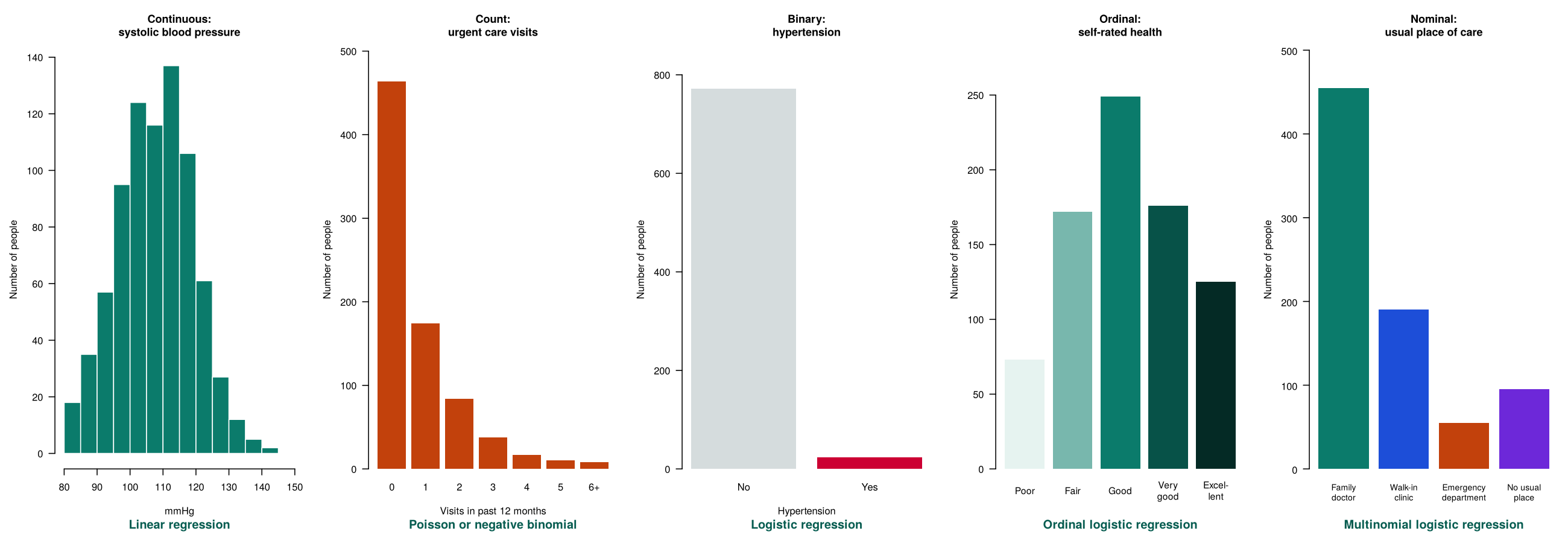
Five outcomes from the PHAA survey
plot(lin) draws the four checks
Introduction and Overview
Regression models describe how an outcome changes with one or more predictors. Lesson 3 introduced two of them: linear regression for a continuous outcome and logistic regression for a binary (yes-or-no) outcome. Many outcomes in public health are neither continuous nor binary. Self-rated health is recorded in ordered categories, the place a person usually goes for care is a choice among unordered options, and the number of emergency visits is a count. This lesson presents one model for each of these outcome types. This first section sets out the types of variables, reviews linear regression and the assumptions on which it rests, and introduces generalized linear models (GLMs), the family to which every model in the lesson belongs.
Learning Objectives
- Classify a variable as continuous, discrete (count), binary, ordinal or nominal.
- State the four assumptions of linear regression and describe how each is checked in R.
- Explain why binary, categorical and count outcomes break the assumptions of linear regression.
- Describe the three parts of a generalized linear model and match each outcome type to a model.
- Fit and check a linear regression and a logistic regression in R.
Box 4.1 reviews four statistical ideas that are needed to read the results in this lesson: confidence intervals, p-values, probability and odds, and exponentiated coefficients. It ends with a retrieval question about an odds ratio that is reported later in this section.
Box 4.1: Background: Statistical foundations
Four ideas are needed to read the results in this lesson.
Confidence intervals. A 95% confidence interval is a range of values calculated from the data. The method that produces it captures the true value in 95% of repeated samples, and the values inside it are those most compatible with the data. For a ratio, an interval that includes 1 shows that the data cannot rule out no association; for a difference, the corresponding value is 0.
p-values. A p-value is the probability of an estimate at least as far from “no association” as the one observed, if there were truly no association. A small p-value shows that the data are hard to reconcile with no association. It is not the probability that the null hypothesis is true, and it does not measure the size or importance of the association.
Probability and odds. The odds of an event are p ÷ (1 − p), and a probability is recovered as odds ÷ (1 + odds). A probability of 0.20 gives odds of 0.25, and odds of 0.25 give back a probability of 0.20. When an event is rare, the odds and the probability are close.
Exponentiated coefficients. A log or logit link puts coefficients on a log scale, where effects add. Exponentiating a coefficient (eβ) turns it into a ratio, such as an odds ratio, on which effects multiply, and the ends of its confidence interval are exponentiated in the same way.
Optional fuller reading: HSCI 341 Lesson 6, Section 4, and the confidence-interval paragraph of the mediation example in HSCI 410 Lesson 1, Section 1.
Retrieval question. Later in this section, smokers have an odds ratio for hypertension of 2.65 (95% CI 1.04 to 6.30). What does the interval show?
Every model in this lesson is chosen according to the type of its outcome. The first step is therefore to identify the type of a variable, which the next part sets out.
Types of Variables
Every variable in a dataset belongs to one of two families. Numeric variables record an amount. They are continuous when any value in a range is possible (blood pressure, body mass index, age measured precisely) and discrete when only whole numbers are possible (the number of visits, cases or falls). Categorical variables place each person into a group. They are nominal when the groups have no natural order (usual place of care, type of cancer, province of residence) and ordinal when the groups have a natural order (self-rated health, pain rated none to severe, stage of disease). A categorical variable with exactly two groups is called binary.
Table 4.1 lists the five types with the family to which each belongs and an example of each from the PHAA data, the survey used throughout this lesson.
Table 4.1. The five types of variable, grouped into two families, with an example of each from the PHAA data.
| Family | Type | What the values look like | Example in the PHAA data |
|---|---|---|---|
| Numeric | Continuous | Any value in a range, including decimals | systolic_bp (mmHg) |
| Numeric | Discrete (count) | Whole numbers 0, 1, 2, and so on | urgent_visits in the past 12 months |
| Categorical | Binary | Two groups | hypertension (No, Yes) |
| Categorical | Ordinal | Three or more groups with a natural order | self_rated_health (Poor to Excellent) |
| Categorical | Nominal | Three or more groups with no order | usual_care (Family doctor, Walk-in clinic, Emergency department, No usual place) |
The type of a variable is decided by what its values mean, and the way it is stored in a file can mislead. Self-rated health might be stored as the numbers 1 to 5, yet it is still ordinal, because the distance between "good" and "very good" is unknown. A postal code is made of characters and numbers, yet it is nominal. The cards below describe each type in more detail.
Worked Example 4.1 applies these definitions to the outcomes of four studies planned by a health unit.
A health unit plans four studies. The first records the number of falls each resident of a care home has in a year, which is a count. The second records whether each resident was admitted to hospital (yes or no), which is binary. The third asks residents how often they feel lonely (never, sometimes, often), which is ordinal. The fourth records the main reason for admission (infection, injury, heart condition, other), which is nominal. Each study therefore needs a different model, even if the predictors are identical.
As Worked Example 4.1 shows, the type of the outcome decides which model is suitable. The next part reviews the model for a continuous outcome, linear regression, and the assumptions on which it rests.
Linear Regression and Its Assumptions
Linear regression models the average of a continuous outcome as a straight-line function of the predictors. For systolic blood pressure (SBP) in the PHAA survey, with age and smoking as predictors, the model is written as in Equation 4.1.
When this model is fitted to the 795 people with complete data, the slope for age is 0.45 mmHg per year (95% CI 0.40 to 0.49) and the difference for smokers is 6.06 mmHg (95% CI 4.33 to 7.79). Activity 4.1 at the end of this section produces these numbers. The estimates can be trusted only if the assumptions below are reasonable. Each assumption is described with the way it is checked in R and with a simple response if it fails.
What it means. The average outcome changes in a straight line as each continuous predictor increases. Blood pressure should rise by about the same amount between ages 30 and 40 as between ages 60 and 70.
How to check it. In the Residuals vs Fitted plot from plot(model), the red smoothed line should be close to flat at zero. A clear curve (a U shape or an arch) suggests that the relationship is not a straight line.
If it fails. A squared term for the predictor, such as I(age^2), can capture a curve, and Lesson 3 showed how to test one.
What it means. Each person's outcome is unrelated to every other person's outcome once the predictors are taken into account.
How to check it. Independence is judged from the study design and cannot be read from a plot. It is usually reasonable when each person is sampled once. It fails when the same person is measured several times, or when people are clustered (patients within clinics, students within schools).
If it fails. Models for dependent data, the topic of Lesson 5, handle repeated or clustered measurements.
What it means. The residuals (each observed value minus the value predicted by the model) follow a roughly bell-shaped distribution. The assumption concerns the residuals, which are checked after the model is fitted, and a skewed outcome can still give normal residuals.
How to check it. In the Q-Q Residuals plot, the points should lie close to the dotted diagonal line. Small wiggles at the ends are common and are not a concern in a large sample.
If it fails. A strongly skewed outcome can sometimes be transformed (for example, by taking its log). If the outcome is a count or a category, a GLM from this lesson is the better choice.
What it means. The residuals are spread about equally across the whole range of predicted values. The technical name for this property is homoscedasticity.
How to check it. In the Residuals vs Fitted and Scale-Location plots, the band of points should have roughly the same height from left to right. A funnel that widens to one side is the usual sign of a problem.
If it fails. Lesson 3 showed sandwich (heteroscedasticity-consistent) standard errors and transformations. When the spread grows with the mean because the outcome is a count, a Poisson or negative binomial model is the better choice.
What it means. No single observation pulls the fitted line far from where the rest of the data would put it.
How to check it. In the Residuals vs Leverage plot, points that fall beyond the dashed Cook's distance lines have large influence. When no point is near them, R does not draw the lines inside the plotting area.
If it fails. The influential record is checked for a data-entry error. If it is a genuine value, the model is reported with and without it.
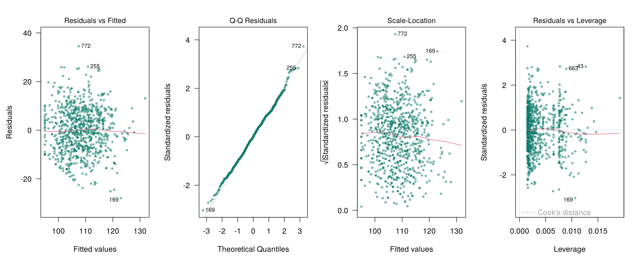
Figure 4.1 shows the four plots that plot(lin) draws for the blood pressure model, so that each of the checks described above can be seen on real output.
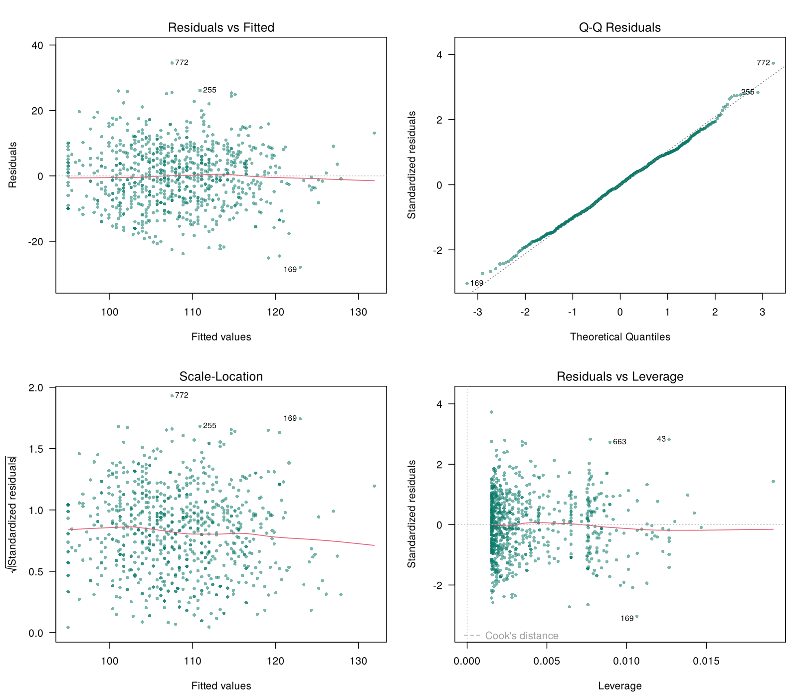
plot(lin) for the blood pressure model. The cloud of residuals is flat and even (linearity and equal variance), the points follow the Q-Q line (normality), and no point lies beyond Cook's distance (no overly influential points). In the first three panels the numbered points are the three largest residuals, and in Residuals vs Leverage they are the three largest Cook's distances; R labels them by row number.For the blood pressure model, the plots in Figure 4.1 support each of the assumptions that a plot can check. The next part turns to outcomes for which these assumptions fail.
Why Some Outcomes Need a Different Model
The same four plots look very different when a straight line is fitted to an outcome that is a count. Figure 4.2 shows the first two plots for a linear regression of urgent_visits (the number of urgent care visits in the past year) on age and smoking.
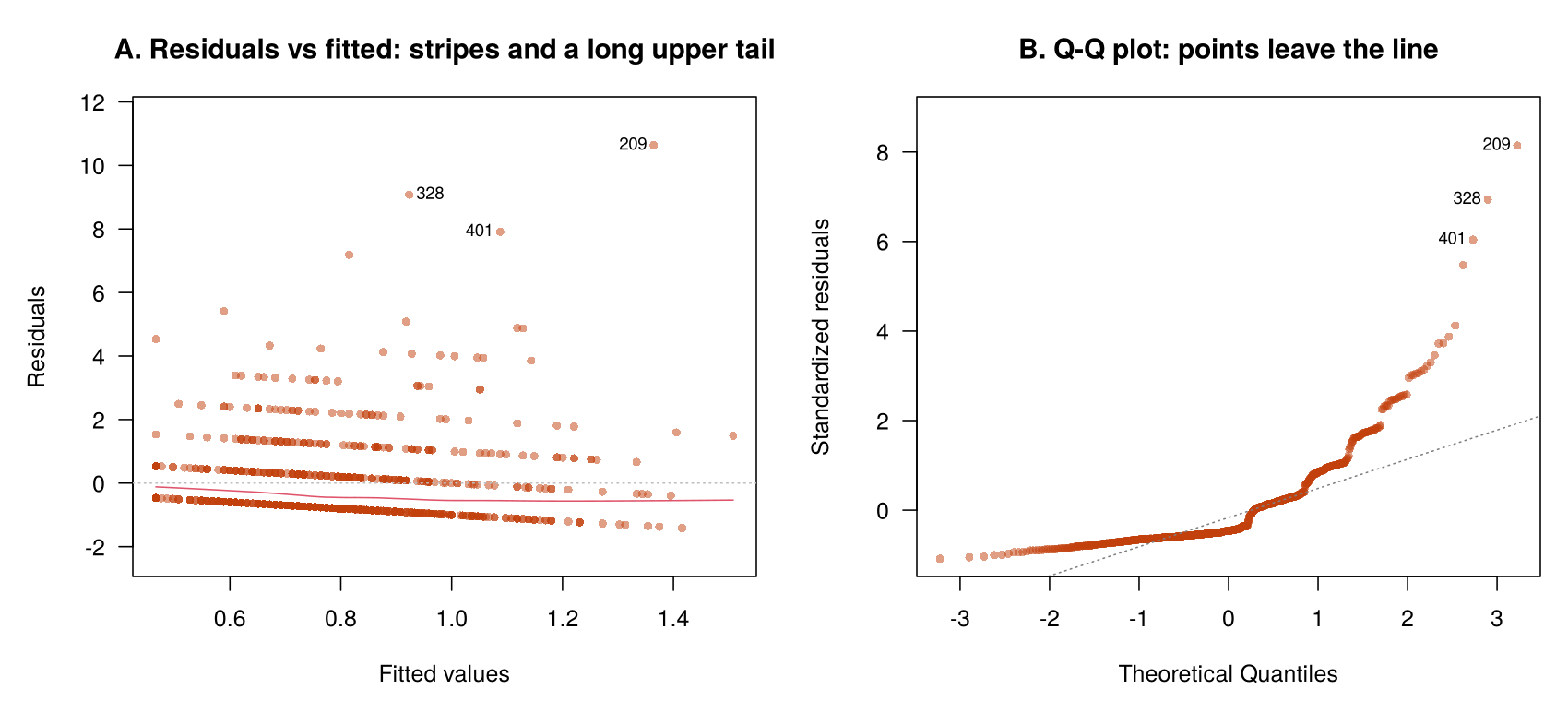
Each outcome type breaks the assumptions in its own way. A binary outcome takes only the values 0 and 1, so a straight line can predict impossible probabilities below 0 or above 1, and the residuals can never be normal. A count cannot be negative, often has many zeros, and becomes more variable as its average increases, which breaks the equal-variance assumption. An ordinal outcome has an order but no known spacing between its categories, so a slope "per category" has no clear meaning. A nominal outcome has no order at all, so any numbers attached to its categories are arbitrary labels.
Linear regression is therefore suited to a continuous outcome, and each of the other four types of outcome calls for a model that matches the values the outcome can take. The next part introduces the family of models that provides one for each type.
Generalized Linear Models
A generalized linear model (GLM) extends linear regression so that it can handle these outcomes. The extension was set out by Nelder and Wedderburn (1972) and is now the standard framework for regression in epidemiology. Every GLM has three parts. The distribution (also called the family) describes the kind of values the outcome can take. The linear predictor is the familiar sum β0 + β1X1 + β2X2 + …, which combines the predictors exactly as in linear regression. The link function is a transformation of the average outcome that is set equal to the linear predictor.
Equation 4.2 shows how the link function connects the average outcome to the linear predictor.
The link function keeps predictions in a sensible range. A probability must lie between 0 and 1, and the logit link guarantees that it does. An expected count must be positive, and the log link guarantees that it is. The link also decides how coefficients are read. When the link is a log or a logit, the coefficient β is on a log scale, so it is exponentiated (eβ, written exp(coef(model)) in R) to turn it into a ratio: an odds ratio, a relative risk ratio or a rate ratio. A ratio of 1 means no association, a ratio above 1 means the outcome is more likely or more frequent, and a ratio below 1 means it is less likely or less frequent.
Table 4.2 lists each model used in this lesson with its type of outcome, its distribution and link, the reading of eβ, and the R function that fits it. The note beneath the table explains why its last row, the Cox model, is included.
Table 4.2. The regression models in this lesson, with the distribution, link, reading of eβ and R function of each.
| Model | Outcome | Distribution | Link | eβ is read as | R function |
|---|---|---|---|---|---|
| Linear regression | Continuous | Normal | Identity (no transformation) | Not exponentiated: β is a difference in means | lm() |
| Logistic regression | Binary | Binomial | Logit | Odds ratio (OR) | glm(family = binomial) |
| Ordinal logistic regression | Ordinal | Multinomial (ordered) | Cumulative logit | Odds ratio for a higher category | MASS:: |
| Multinomial logistic regression | Nominal | Multinomial | Logit versus a reference category | Relative risk ratio (RRR) | nnet:: |
| Poisson regression | Count | Poisson | Log | Incidence rate ratio (IRR) | glm(family = poisson) |
| Negative binomial regression | Overdispersed count | Negative binomial | Log | Incidence rate ratio (IRR) | MASS:: |
| Cox proportional hazards model | Time to event (with censoring) | None assumed for the baseline hazard | Log of the hazard | Hazard ratio (HR) | survival:: |
Strictly, the ordinal and multinomial models are close relatives of the GLM family (they are often called multivariate GLMs), because they model several probabilities at once. They are fitted and read in the same way, and this course treats them as members of the family. The Cox model in the last row is not a GLM, because it leaves the shape of the baseline hazard unspecified. It is listed because a time-to-event outcome is one more outcome type, and it is covered only in the optional Survival Analysis in R walkthrough linked below.
Table 4.2 pairs each type of outcome with a model. The next part turns this pairing into a short guide for choosing a model.
Choosing a Model
The choice of model follows from the type of the outcome, and the predictors play no part in it. The guide in Figure 4.3 can be worked through for any new outcome. The first question is whether the outcome is numeric or categorical, and the second question narrows the choice to one model.
Figure 4.3. A decision guide that leads from the type of the outcome to a model, with one column for numeric outcomes and one for categorical outcomes.
The last row of the numeric column in Figure 4.3 leads to the Cox model, which the note to Table 4.2 places outside the GLM family. Box 4.2 defines the terms used for time-to-event outcomes, and the card that follows it links to the optional Survival Analysis in R walkthrough.
Box 4.2: Background: Time-to-event outcomes
Some outcomes record how long each person is followed until an event occurs, such as death, relapse or a first hospital admission. Five terms describe these data.
- Time zero is the moment from which follow-up time is counted for every person, such as diagnosis, enrolment or the start of treatment.
- Censoring occurs when a person’s follow-up ends before the event is observed, because the study ends, the person withdraws or they are lost to follow-up. Their time to the event is known only to be longer than the time observed.
- The survival curve shows the estimated proportion of people still free of the event at each time after time zero. The Kaplan-Meier method estimates it and uses the follow-up of censored people up to the time they leave.
- The hazard is the rate at which the event occurs at a given time among the people still at risk, that is, still under follow-up and still free of the event.
- The hazard ratio compares the hazards of two groups. A hazard ratio of 2 means that, among people still at risk, one group has the event at twice the rate of the other. The Cox proportional hazards model estimates hazard ratios and assumes that each ratio stays constant over follow-up.
An ordinary average of follow-up times, or the proportion of people with the event, gives the wrong answer when some follow-up is incomplete, which is why these outcomes need their own methods. For fuller treatments (optional reading), see HSCI 341 Lesson 8 (Time-to-Event Data) and the concept primer at the start of the Survival Analysis in R walkthrough below.
Narrated R walkthrough: Survival Analysis in R
Some outcomes record how long people are followed until an event occurs, and some people leave the study before the event is observed. These time-to-event outcomes need survival methods. This walkthrough introduces time zero, events and censoring, and then fits Kaplan-Meier curves, a log-rank test and a Cox proportional hazards model to the lung cancer data that come with the survival package.
Open the Survival Analysis in R walkthroughWith a model matched to each type of outcome, the rest of this section reviews logistic regression, the model for a binary outcome that Lesson 3 introduced. Sections 2, 3 and 4 then take up the ordinal, nominal and count models in turn.
Logistic Regression: A Brief Review
Logistic regression is the GLM for a binary outcome. It models the log of the odds of the event, and its exponentiated coefficients are odds ratios (Lesson 3 covers it in detail). In the PHAA data, the odds of hypertension are 2.65 times as high for smokers as for non-smokers of the same age (95% CI 1.04 to 6.30), and they are 1.05 times as high (about 5% higher) for each additional year of age (95% CI 1.01 to 1.08). Its assumptions differ from those of linear regression, because a binary outcome has no normal residuals and no constant spread to check.
Table 4.3 lists the assumptions of logistic regression with the way each is checked.
Table 4.3. The assumptions of logistic regression and how each is checked.
| Assumption | What it means | How to check it |
|---|---|---|
| Binary outcome | The outcome has exactly two categories. | table(outcome) shows two groups. |
| Independence | Each person contributes one independent observation. | Judged from the study design. |
| Linearity in the log-odds | Each continuous predictor has a straight-line relationship with the log-odds of the event. | Add a squared term (for example I(age^2)) and check whether it improves the model, as shown in Lesson 3. |
| Enough events | A common rule of thumb asks for about 10 events per predictor. | table(outcome) gives the number of events. With 23 events, about two predictors are supported. |
| No strong multicollinearity | Predictors are not so strongly related that their effects cannot be separated. | Correlations among predictors, or variance inflation factors as in Lesson 3. |
The rule of about 10 events per predictor in Table 4.3 matters in the PHAA data, because few participants have hypertension. Box 4.3 explains how the small number of events affects the confidence interval for smoking.
Box 4.3: Why the confidence interval for smoking is wide
Only 23 of the 795 people have hypertension. With so few events, the model has little information about each predictor, and the 95% confidence interval for the smoking odds ratio runs from 1.04 to 6.30. The point estimate of 2.65 suggests a strong association, but the data are consistent with anything from a very small increase to a six-fold increase in the odds. Reporting the interval alongside the estimate makes this uncertainty visible to readers.
Once a model has been fitted and checked, its results are usually reported in a table. Box 4.4 shows how the output of the logistic model becomes a results table of the kind found in published papers.
Box 4.4: From Model Output to a Results Table
Published papers usually report a regression in a table that sets the crude (unadjusted) estimate for each predictor beside the adjusted estimate from the multivariable model, so that readers can see how much adjustment changed each association. The crude odds ratio for a predictor comes from a logistic model with that predictor alone, such as glm(hypertension ~ smoker, data = phaa, family = binomial), and the adjusted odds ratios come from the model with age and smoking together. For the PHAA example, Table 4.4 reads as follows.
Table 4.4. Crude and adjusted odds ratios for hypertension in the PHAA example.
| Predictor | Crude OR (95% CI) | Adjusted OR (95% CI) |
|---|---|---|
| Age (per year) | 1.05 (1.01 to 1.08) | 1.05 (1.01 to 1.08) |
| Smoker (yes vs. no) | 2.76 (1.09 to 6.50) | 2.65 (1.04 to 6.30) |
Odds ratios for hypertension among the 795 PHAA participants with complete data (23 events). The adjusted odds ratios come from one logistic regression that includes age and smoking. The 95% confidence intervals come from confint().
A clear results table states the outcome, the number of people and events, the reference category of each categorical predictor, the unit of each continuous predictor and the variables in the adjusted model. In this example adjustment changes the smoking odds ratio only slightly, from 2.76 to 2.65, because smokers and non-smokers in these data have almost the same average age (45.5 and 45.1 years).
This section has matched each type of outcome to a model and reviewed the two models from Lesson 3. The two R activities below put this review into practice. Activity 4.1 fits the linear model for systolic blood pressure and draws the plots in Figure 4.1, and Activity 4.2 fits the logistic model for hypertension and produces the adjusted odds ratios in Table 4.4. A knowledge check and a reflection close the section.
This activity fits the linear model for systolic blood pressure and runs its checks. Download phaa_outcomes.csv and save it in the folder that holds your R script. In RStudio, choose Session → Set Working Directory → To Source File Location so that R can find the file. The file holds the 800 PHAA participants, and the code keeps the 795 people with no missing values, so that every model in this lesson uses the same people.
# install.packages(c("MASS", "nnet", "brant"))   # run once, if not yet installed
phaa <- read.csv("phaa_outcomes.csv")   # file must be in the working directory
phaa <- na.omit(phaa)                   # keep the 795 people with no missing values
phaa$smoker <- factor(phaa$smoker, levels = c("No", "Yes"))   # "No" = reference
nrow(phaa)                   # how many people are in the analysis?
summary(phaa$systolic_bp) # a first look at the outcomeThe nrow() line confirms that 795 people are in the analysis. Systolic blood pressure ranges from 85 to 145 mmHg, with a mean of 108.2 and a median of 109, so the mean and the median are close, which is what a roughly symmetric outcome looks like.
lin <- lm(systolic_bp ~ age + smoker, data = phaa)   # fit the linear model
summary(lin)                 # coefficients, standard errors and p-values
confint(lin) # 95% confidence intervalsReading the output. The Estimate column holds the coefficients. The intercept (86.93) is the predicted blood pressure for a non-smoker aged 0, which is outside the data and has no practical meaning. The age slope (0.447) means that blood pressure is 0.45 mmHg higher, on average, for each extra year of age, holding smoking constant. The smoking coefficient (6.06) means that smokers average 6.06 mmHg higher than non-smokers of the same age. Both p-values are far below 0.05. Multiple R-squared (0.33) says that age and smoking together explain about a third of the variation in blood pressure. The confint() table gives the 95% confidence intervals: 0.40 to 0.49 for age and 4.33 to 7.79 for smoking.
par(mfrow = c(2, 2))         # show four plots on one screen
plot(lin)                    # the four standard checks of a linear model
par(mfrow = c(1, 1))         # back to one plot per screen
These three lines produce no console output. They draw the four diagnostic plots shown in Figure 4.1. Compare your plots with that figure: a flat red line in Residuals vs Fitted, points close to the line in Q-Q Residuals, an even band in Scale-Location, and no points beyond Cook's distance in Residuals vs Leverage.
R Reflect on what you just ran
Use the questions below to interpret the output you produced. Look at your console output and plots before answering.
1. From summary(lin), report the coefficient for smokerYes with its 95% confidence interval from confint(lin), and write one sentence that explains what it means.
2. Look at the Residuals vs Fitted and Q-Q Residuals plots. Which assumptions does each plot check, and do they look acceptable for this model?
3. Which of the four LINE assumptions cannot be checked with these plots, and how would you decide whether it holds in the PHAA survey?
This activity reviews logistic regression with the same predictors. The first lines load the data again, so the activity can be run on its own.
phaa <- read.csv("phaa_outcomes.csv")   # file must be in the working directory
phaa <- na.omit(phaa)                   # keep the 795 people with no missing values
phaa$smoker <- factor(phaa$smoker, levels = c("No", "Yes"))   # "No" = reference
phaa$hypertension <- factor(phaa$hypertension, levels = c("No", "Yes"))   # "Yes" is the event
table(phaa$hypertension) # check: how many people had the event?The first check for a logistic regression is the number of events. Here 23 of the 795 people have hypertension. With the rule of thumb of about 10 events per predictor, 23 events support a model with about two predictors, which is what this model has.
logit <- glm(hypertension ~ age + smoker, data = phaa, family = binomial)
summary(logit)
exp(cbind(OR = coef(logit), confint(logit))) # odds ratios with 95% CIsReading the output. The Estimate column is on the log-odds scale, so the last line exponentiates the coefficients to give odds ratios. The odds ratio for age is 1.045 (95% CI 1.014 to 1.078): each extra year of age multiplies the odds of hypertension by about 1.05, which is about 5% higher odds. The odds ratio for smoking is 2.65 (95% CI 1.04 to 6.30): smokers have about 2.6 times the odds of hypertension of non-smokers of the same age. The odds ratio for the intercept is the odds of hypertension for a non-smoker aged 0 and is not interpreted.
R Reflect on what you just ran
Use the questions below to interpret the output you produced. Look at your console output before answering.
1. Report the odds ratio for smokerYes with its 95% confidence interval, and explain it in one sentence.
2. Using the output of table(phaa$hypertension), explain whether this dataset has enough events to add three more predictors (for example BMI, gender and income) to the model.
3. Why would it be inappropriate to check this logistic model with a Q-Q plot of the residuals, as was done for the linear model?
1. A researcher records the number of asthma attacks each child has during a school year. What type of variable is this?
2. Which variable is ordinal?
3. Which of the following is an assumption of linear regression that is checked with a Q-Q plot of the residuals?
4. In a generalized linear model, what does the link function do?
5. A logistic regression has 30 events. Using the rule of thumb of about 10 events per predictor, how many predictors can the model support?
✎ Reflection
This section described five types of outcome: continuous (any value in a range, such as blood pressure), discrete counts (whole numbers such as the number of visits), binary (two groups, such as hypertension yes or no), ordinal (ordered groups, such as self-rated health from poor to excellent) and nominal (unordered groups, such as usual place of care). It paired them with linear regression, Poisson or negative binomial regression, logistic regression, ordinal logistic regression and multinomial logistic regression respectively. It also described the four assumptions of linear regression: linearity, independence, normality of the residuals and equal variance. Choose one health outcome from an area of public health that interests you. Name the outcome, state its type and the model that suits it, and explain which of the four linear regression assumptions the outcome would break if it were analysed with a straight-line model.
Ordinal Logistic Regression
Self-rated health by smoking
Introduction and Overview
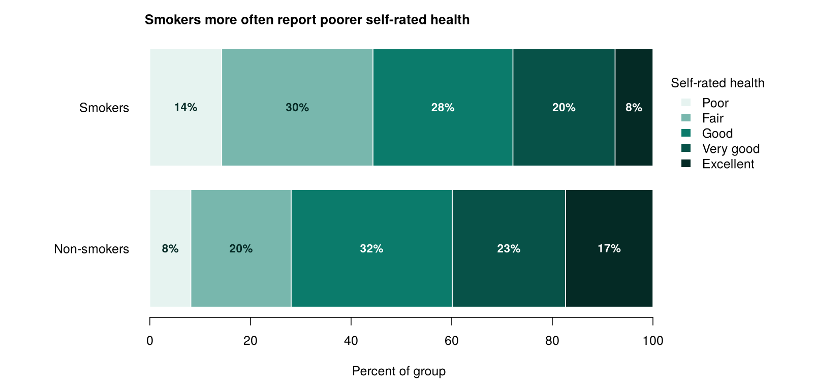
This section presents ordinal logistic regression, the model for an outcome with three or more ordered categories. The running example is self-rated health, a widely used single question in health surveys that asks people to rate their own health as poor, fair, good, very good or excellent. Self-rated health predicts later illness and death even after other measures of health are taken into account (Idler & Benyamini, 1997), which makes it a common outcome in public health research. In the PHAA data, self-rated health is a simulated variable added for this lesson. The section fits the model with age and smoking as predictors and checks its assumptions.
Learning Objectives
- Recognize an ordinal outcome and explain why linear regression and binary logistic regression are poor choices for it.
- Describe how the ordinal model compares "at or above" with "below" at each split of the outcome.
- Fit an ordinal logistic regression in R with
polr()and interpret its odds ratios. - Check the proportional-odds assumption with the Brant test and name what to do if it fails.
The section begins by setting out what makes an outcome ordinal and why the two common ways of simplifying such an outcome lose information.
What Makes an Outcome Ordinal?
An outcome is ordinal when its categories can be ranked but the distances between them are unknown. Self-rated health, pain severity, agreement scales, disease stage and education level are all ordinal. The defining feature is that the order carries information: a move from "good" to "very good" is a move in a known direction. What the order does not say is how large each move is. The step from "poor" to "fair" might reflect a much larger change in health than the step from "very good" to "excellent", and the data offer no way to measure the difference.
Two shortcuts are common in practice, and both lose something. Coding the categories as 1 to 5 and fitting a linear regression treats every step as equal and assumes normal residuals, which a five-category outcome cannot have. Collapsing the categories into two groups and fitting a logistic regression discards the detail within each group and makes the result depend on where the cut-off is placed. Ordinal logistic regression avoids both problems.
The three cards below set the two shortcuts beside ordinal logistic regression, so that what each approach assumes and what it loses can be compared.
Ordinal logistic regression keeps every category and uses their order. The next part shows how it does this by fitting a series of splits of the outcome.
How the Model Works: A Series of Splits
An outcome with five ordered categories can be split into "at or above" and "below" in four places. Each split is a yes-or-no comparison that a binary logistic regression could handle on its own. The ordinal model fits the four comparisons together.
Figure 4.4 shows the four splits for self-rated health.
Figure 4.4. The four splits of the five categories of self-rated health, each comparing the categories at or above the split with those below it.
The model gives each split its own intercept, because the proportion of people at or above the split differs from one split to the next: almost everyone is "fair or better", while only a small share is "excellent". Each predictor, however, receives a single coefficient that applies to every split. This is why the model is called the proportional-odds model, and it is the assumption that the Brant test checks later in this section (McCullagh, 1980).
Equation 4.3 writes the model for self-rated health with age and smoking as predictors.
Box 4.5 explains how R writes this model and what that means for the sign of each coefficient and for the intercepts.
⚠ Box 4.5: How R writes the model
Some textbooks and software write the ordinal model the other way round, as the odds of being at or below a category, which flips the sign of every coefficient. R's polr() is set up so that a positive coefficient means that higher categories are more likely and a negative coefficient means that lower categories are more likely. With self-rated health ordered from Poor to Excellent, an odds ratio below 1 therefore means poorer reported health. The order of the levels in factor() decides which end of the scale counts as "higher", so it is worth checking that order before reading any result. R also prints the intercepts (cut-points) with the opposite sign to β0j in Equation 4.3, so they cannot be substituted into that formula directly.
Worked Example 4.2 calculates the crude odds ratio for smoking at each of the four splits in Figure 4.4, so that the single odds ratio estimated by the model can be set beside the split-specific values.
Worked Example 4.2: The Four Splits by Hand
The table in Activity 4.3 below gives the number of non-smokers and smokers in each category. Non-smokers (n = 662) are spread as 54 poor, 132 fair, 212 good, 149 very good and 115 excellent. Smokers (n = 133) are spread as 19 poor, 40 fair, 37 good, 27 very good and 10 excellent.
At split 2 (good or better versus poor or fair), 476 non-smokers are at or above the split and 186 are below it, so their odds are 476 ÷ 186 = 2.56. For smokers, 74 are at or above and 59 are below, so their odds are 74 ÷ 59 = 1.25. The crude odds ratio at this split is 1.25 ÷ 2.56 = 0.49. Repeating the arithmetic at the other splits gives crude odds ratios of 0.53 at split 1, 0.58 at split 3 and 0.39 at split 4.
The four crude odds ratios are similar, and they all point in the same direction. The ordinal model replaces them with one number, 0.50, which also adjusts for age. The Brant test asks whether the four split-specific values differ by more than chance would produce.
The next part reads the single odds ratio for smoking, and the rest of the output, from the model fitted to the PHAA data.
Interpreting the Results
Fitted to the 795 people in the PHAA data, the ordinal model gives an odds ratio for smoking of 0.50 (95% CI 0.36 to 0.70). Smokers have about half the odds of non-smokers of the same age of reporting a higher category of self-rated health, and the model applies this odds ratio at every split. The odds ratio for age is 0.966 per year (95% CI 0.957 to 0.975). Because one year is a small step, the odds ratio for ten years is easier to picture: 0.96610 = 0.71, so a person ten years older has about 29% lower odds of reporting a higher category. In R, the ten-year odds ratio is exp(10 * coef(ord)["age"]).
The output of polr() also lists four intercepts, labelled Poor|Fair, Fair|Good, Good|Very good and Very good|Excellent. These are the cut-points between neighbouring categories. They are needed to calculate predicted probabilities, but they are not usually reported or interpreted. The output gives t values but no p-values. The 95% confidence intervals from confint() answer the same question: when an interval for an odds ratio excludes 1, the association is statistically significant at the 5% level.
Figure 4.5 shows the distribution of self-rated health among non-smokers and smokers that lies behind the odds ratio for smoking.
These odds ratios can be trusted only if the assumptions of the model are reasonable, and the next part turns to those assumptions.
Assumptions and How to Check Them
The ordinal model shares the general assumptions of logistic regression and adds one of its own. Table 4.5 lists each assumption with the way it is checked.
Table 4.5. The assumptions of ordinal logistic regression and how each is checked.
| Assumption | What it means | How to check it |
|---|---|---|
| Ordered outcome | The categories have a genuine, meaningful order. | Reasoning about the categories; the levels are set in order with factor(…, ordered = TRUE). |
| Independence | Each person contributes one independent observation. | Judged from the study design. |
| Enough people in each category | No category is nearly empty, overall or within the groups of a categorical predictor. | table(outcome) and table(predictor, outcome). |
| No strong multicollinearity | The predictors are not so strongly related that their effects cannot be separated. | Correlations among the predictors. |
| Proportional odds | Each predictor has the same odds ratio at every split of the outcome. | brant(model) from the brant package (Brant, 1990). |
The proportional-odds assumption in the last row of Table 4.5 is the one that the ordinal model adds. The accordion below explains how the Brant test checks it and what can be done if it fails.
The Brant test fits a separate binary logistic regression at each split and compares the coefficients across the splits. If the proportional-odds assumption holds, the coefficients should be similar apart from chance variation. The test reports an omnibus result for all predictors together and one result for each predictor. Each result is a chi-squared statistic with a p-value. A p-value above 0.05 means that the data are consistent with the assumption, and a p-value below 0.05 means that the predictor's odds ratio appears to change from one split to another.
There are three common responses. When a failure is driven by a category with very few people, combining it with a neighbouring category (for example, poor with fair) can solve the problem, provided the combined category still makes sense. When the assumption fails badly, the order can be set aside and a multinomial logistic regression fitted (Section 3), which gives each category its own relative risk ratios. When only one or two predictors fail, a partial proportional-odds model lets those predictors have a different odds ratio at each split while keeping one odds ratio for the others. Partial proportional-odds models are fitted with the vglm() function in the VGAM package and are beyond the scope of this course. In very large samples the Brant test can flag small differences that have no practical importance, so the split-specific odds ratios are worth inspecting before the model is abandoned.
This section has shown how the ordinal model is fitted, read and checked. The card below links to a narrated walkthrough of ordinal logistic regression in R, and Activity 4.3 fits the model of this section to the PHAA data, reproduces its odds ratios and runs the Brant test. A knowledge check and a reflection close the section.
Narrated R walkthrough: Ordinal Logistic Regression in R
This walkthrough fits an ordinal logistic regression to the course outcomes data. It orders the outcome categories, looks at the data before modelling, converts the results to odds ratios and predicted probabilities, and checks the proportional odds assumption.
Open the Ordinal Logistic Regression in R walkthroughThis activity fits the ordinal model for self-rated health and checks the proportional-odds assumption. It needs the MASS package, which is installed with R, and the brant package, which may need to be installed once with install.packages("brant").
library(MASS)    # polr() fits the ordinal logistic model
library(brant)   # brant() checks the proportional-odds assumption
phaa <- read.csv("phaa_outcomes.csv")   # file must be in the working directory
phaa <- na.omit(phaa)                   # keep the 795 people with no missing values
phaa$smoker <- factor(phaa$smoker, levels = c("No", "Yes"))   # "No" = reference
phaa$self_rated_health <- factor(phaa$self_rated_health,
  levels = c("Poor", "Fair", "Good", "Very good", "Excellent"), ordered = TRUE)
table(phaa$smoker, phaa$self_rated_health) # check: people in each category, by smokingThe factor() line sets the order of the categories from Poor to Excellent and marks the variable as ordered, which polr() needs. The table is the first check: every category has people in it in both smoking groups, and the smallest cell (10 smokers who rate their health as excellent) is small but not empty.
ord <- polr(self_rated_health ~ age + smoker, data = phaa, Hess = TRUE)
summary(ord)Reading the output. The Coefficients block holds one value per predictor on the log-odds scale. Both are negative, which with polr() means that older people and smokers are more likely to be in the lower (poorer) categories. The Intercepts block holds the four cut-points between neighbouring categories, which are not usually interpreted. The model reports t values but no p-values, so the confidence intervals in the next step are used to judge significance.
exp(cbind(OR = coef(ord), confint(ord))) # odds ratios with 95% CIsExponentiating gives odds ratios. The odds ratio for smoking is 0.50 (95% CI 0.36 to 0.70), so smokers have half the odds of non-smokers of the same age of reporting a higher category. The odds ratio for age is 0.966 per year (95% CI 0.957 to 0.975), or 0.71 per ten years. Both intervals exclude 1.
brant(ord) # check the proportional-odds assumptionThe Brant test reports an omnibus p-value of 0.35 and p-values of 0.23 for age and 0.53 for smoking. All are above 0.05, so the proportional-odds assumption is reasonable for this model. The last line of the output states the null hypothesis that is being tested: that the assumption (called the parallel regression assumption) holds.
R Reflect on what you just ran
Use the questions below to interpret the output you produced. Look at your console output before answering.
1. Report the odds ratio for smokerYes with its 95% confidence interval, and write one sentence that explains it in terms of self-rated health.
2. The odds ratio for age is 0.966. Calculate the odds ratio for a ten-year difference in age and explain what it means.
exp(10 * -0.03421) = 0.71). A person who is ten years older than another person with the same smoking status has about 0.71 times the odds, or about 29% lower odds, of reporting a higher category of self-rated health.3. Using the output of brant(ord), state whether the proportional-odds assumption holds and give the evidence. What would you do if the p-value for smoking had been 0.01?
1. Which outcome is best analysed with ordinal logistic regression?
2. An ordinal outcome has four categories. How many splits (and intercepts) does the ordinal logistic model use?
3. What is the proportional-odds assumption?
4. In a polr() model of self-rated health (ordered Poor to Excellent), the odds ratio for regular physical activity is 1.8. What does this mean?
polr(), an odds ratio above 1 means that higher categories are more likely. An odds ratio of 1.8 means 1.8 times the odds of being in a higher category, at every split.5. The Brant test for a model gives an omnibus p-value of 0.002. What does this suggest?
✎ Reflection
This section showed that ordinal logistic regression (the proportional-odds model, fitted with polr() in R) suits an outcome with three or more ordered categories. It fits every "at or above versus below" split of the outcome at once and gives each predictor a single odds ratio for being in a higher category. Its special assumption, that each predictor has the same odds ratio at every split, is checked with the Brant test, where a p-value above 0.05 means the data are consistent with the assumption. In the PHAA data, smokers had an odds ratio of 0.50 (95% CI 0.36 to 0.70) for reporting a higher category of self-rated health. Suppose a colleague proposes coding self-rated health as 1 to 5 and using linear regression instead, because "the numbers are easier to explain". Write a short reply that explains, in plain language, what the linear approach would assume about the categories, what the ordinal model offers in its place, and how you would describe the smoking result to a non-specialist audience.
Multinomial Logistic Regression
Usual place of care by smoking
Introduction and Overview
This section presents multinomial logistic regression, the model for an outcome with three or more categories that have no natural order. The running example is the usual place of care, a question asked in many Canadian health surveys because having a regular source of primary care is linked to better access to preventive services and continuity of care. In the PHAA data, usual place of care is a simulated variable added for this lesson, with four categories: family doctor, walk-in clinic, emergency department and no usual place. The section fits the model with age and smoking as predictors, interprets its relative risk ratios and predicted probabilities, and lists the assumptions to check.
Learning Objectives
- Recognize a nominal outcome and explain why the ordinal model does not suit it.
- Explain the role of the reference category and why a K-category outcome gives K − 1 comparisons.
- Fit a multinomial logistic regression in R with
multinom()and interpret its relative risk ratios. - Calculate and present predicted probabilities from the model.
- List the assumptions of the multinomial model, including the independence of irrelevant alternatives.
The section begins with what makes an outcome nominal and why such an outcome needs a model of its own.
What Makes an Outcome Nominal?
An outcome is nominal when its categories are simply different from one another, with no ranking. A family doctor, a walk-in clinic and an emergency department are different kinds of places, and none of them is "more" than the others. Type of cancer, main mode of travel to work, type of nicotine product and reason for missing a vaccination are other examples. Because there is no order to use, a model for a nominal outcome must let each category have its own relationship with every predictor.
A smoker might be more likely than a non-smoker to use an emergency department and also more likely to have no usual place, and the two increases need not be the same size. An ordinal model, which gives each predictor a single odds ratio for "moving up the scale", cannot describe this pattern, because there is no scale to move along.
The next part shows how the multinomial model gives each category its own coefficients by comparing it with a reference category.
How the Model Works: Comparisons With a Reference Category
The multinomial model chooses one category as the reference category and compares every other category with it. In R, the reference is set with relevel(), and this lesson uses family doctor, the most common answer. Figure 4.6 sets out the comparisons that follow from this choice. With four categories, the model makes three comparisons:
Figure 4.6. The three comparisons that the multinomial model makes for usual place of care, each with family doctor as the reference category.
In general, an outcome with K categories gives K − 1 comparisons. Each comparison is written like a small logistic regression, with its own intercept and its own slope for every predictor (Hosmer, Lemeshow & Sturdivant, 2013). The model fits all of the comparisons at the same time, so that the predicted probabilities of the four categories always add to 1.
Equation 4.4 writes the model for each comparison with the reference category, with age and smoking as predictors.
The choice of reference category changes how the results are presented. It does not change how well the model fits or the predicted probabilities. A different reference (for example, walk-in clinic) would give a different set of comparisons from the same fitted model. A good reference category is a large group that is a natural point of comparison for the research question.
Each comparison has its own coefficients, and the next part shows how their exponentiated values are read.
Interpreting the Results: Relative Risk Ratios
The exponentiated coefficients of a multinomial model are called relative risk ratios (RRRs). Each RRR describes one comparison. For smoking in the emergency department comparison, the RRR says how many times larger the ratio P(emergency department) ÷ P(family doctor) is for smokers than for non-smokers of the same age. An RRR above 1 means that the predictor is associated with a higher chance of the category relative to the reference, and an RRR below 1 means that it is associated with a lower chance of the category relative to the reference.
Worked Example 4.3 calculates a crude RRR for smoking from the counts in the PHAA data and compares it with the RRR from the model.
Worked Example 4.3: A Relative Risk Ratio by Hand
The cross-table in Activity 4.4 below shows 399 non-smokers and 56 smokers with a family doctor, and 39 non-smokers and 16 smokers who name an emergency department. Among smokers, the ratio of emergency department to family doctor is 16 ÷ 56 = 0.286. Among non-smokers, the same ratio is 39 ÷ 399 = 0.098. The crude RRR is 0.286 ÷ 0.098 = 2.92.
The model's RRR for this comparison is 3.01. It differs slightly from the crude value because the model also adjusts for age. The same arithmetic gives crude RRRs of 2.54 for no usual place (25 ÷ 56 compared with 70 ÷ 399) and 1.67 for a walk-in clinic (36 ÷ 56 compared with 154 ÷ 399).
Table 4.6 gives the RRRs from the fitted model for smoking and for age in each of the three comparisons.
Table 4.6. Relative risk ratios for usual place of care from the multinomial model, with family doctor as the reference category.
| Comparison (versus Family doctor) | RRR for smokers (95% CI) | RRR per year of age (95% CI) | RRR per 10 years of age |
|---|---|---|---|
| Walk-in clinic | 1.72 (1.08 to 2.74) | 0.977 (0.96 to 0.99) | 0.79 |
| Emergency department | 3.01 (1.57 to 5.75) | 0.983 (0.96 to 1.00) | 0.84 |
| No usual place | 2.66 (1.54 to 4.61) | 0.960 (0.94 to 0.98) | 0.66 |
Smoking is associated with all three comparisons: among people of the same age, smokers are more likely than non-smokers to name a walk-in clinic, an emergency department or no usual place, each compared with a family doctor. Age is clearly associated with two of the comparisons. Older people are less likely to use a walk-in clinic (RRR 0.79 per ten years) or to have no usual place (RRR 0.66 per ten years), each compared with having a family doctor. The interval for the emergency department comparison includes 1, so the data do not show a clear age difference for that comparison. The ten-year values are calculated from the unrounded coefficients, for example exp(10 * coef(mn)[, "age"]).
Box 4.6 explains what an RRR describes and what it leaves out.
⚠ Box 4.6: An RRR is a ratio of two ratios
An RRR compares one category with the reference only. The RRR of 3.01 describes the ratio of emergency department to family doctor, which is three times as large for smokers as for non-smokers. The overall chance that a smoker names an emergency department is a different quantity, and the predicted probabilities in Table 4.7 show it.
The next part turns to these predicted probabilities.
Predicted Probabilities
The predict() function converts the fitted model into the probability of each category for any chosen combination of predictor values. Predicted probabilities are often the clearest way to present a multinomial model to readers who are not statisticians. Table 4.7 shows them for two 30-year-olds who differ only in smoking status.
Table 4.7. Predicted probabilities of each usual place of care for a non-smoker and a smoker aged 30.
| Person | Family doctor | Walk-in clinic | Emergency department | No usual place |
|---|---|---|---|---|
| Non-smoker, age 30 | 0.51 | 0.28 | 0.06 | 0.15 |
| Smoker, age 30 | 0.32 | 0.30 | 0.12 | 0.26 |
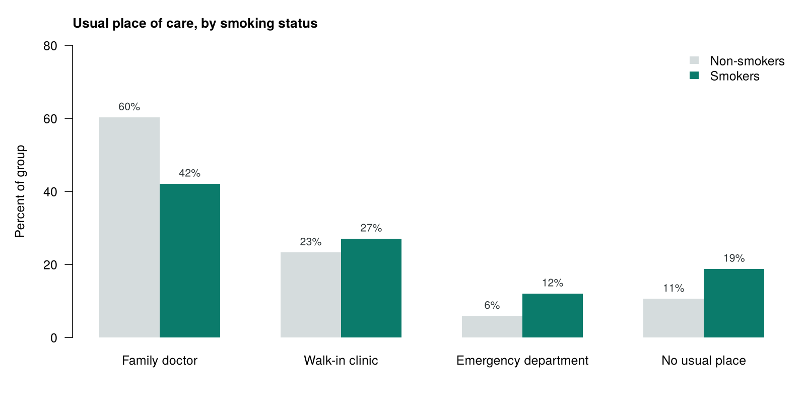
For the 30-year-old smoker, the probability of naming an emergency department (0.12) is twice that for the non-smoker (0.06), and the probability of having no usual place rises from 0.15 to 0.26. These numbers can be stated directly in a report: in this population, about one in four 30-year-old smokers has no usual place of care.
Figure 4.7 shows the observed percentages in each category by smoking status, for all ages combined, which can be set beside the predicted probabilities in Table 4.7.
The relative risk ratios and predicted probabilities can be trusted only if the assumptions of the model hold, and the next part sets them out.
Assumptions and How to Check Them
Table 4.8 lists the assumptions of the multinomial model with the way each is checked. The first four resemble the assumptions of the ordinal model in Table 4.5 in Section 2, and the last, the independence of irrelevant alternatives (IIA), is new.
Table 4.8. The assumptions of multinomial logistic regression and how each is checked.
| Assumption | What it means | How to check it |
|---|---|---|
| Nominal, mutually exclusive categories | The categories have no meaningful order, and each person belongs to exactly one. | Reasoning about the categories and the survey question. |
| Independence | Each person contributes one independent observation. | Judged from the study design. |
| Enough people in every category | Each comparison is estimated separately, so a small category gives unstable estimates and wide intervals. | table(outcome) and table(outcome, predictor). Very small categories can sometimes be combined with a similar category. |
| No strong multicollinearity | The predictors are not so strongly related that their effects cannot be separated. | Correlations among the predictors. |
| Independence of irrelevant alternatives (IIA) | The comparison between any two categories does not depend on which other categories are available. | Reasoning about whether any two categories are close substitutes. Formal tests exist but are beyond the scope of this course. |
The accordion below explains the IIA assumption with an example and sets out why the multinomial model needs more data than the ordinal model.
The IIA assumption says that the odds of choosing one category over another stay the same whether or not other categories are on offer. A classic illustration involves travel to work. Suppose people choose between a car and a red bus, with even odds. If a blue bus that is identical to the red bus is added, common sense says that the new bus takes riders mainly from the red bus, while the multinomial model assumes that it takes riders evenly from both the car and the red bus. The assumption fails because the two buses are near-perfect substitutes. In the PHAA example, a family doctor, a walk-in clinic, an emergency department and no usual place are distinct kinds of care, so the assumption is reasonable. It would be less reasonable if the categories included two very similar options, such as two walk-in clinics run by the same provider.
The multinomial model estimates a separate set of coefficients for every comparison. In this example, two predictors and three comparisons give six slopes and three intercepts, nine numbers in all (R reports # weights: 16 (9 variable) when trace = TRUE). An ordinal model for an outcome with the same number of categories would estimate two slopes and three cut-points. Each extra number is estimated with less information, so small categories produce wide confidence intervals. The emergency department category, with 55 people, has the widest intervals in this example.
With both models for categorical outcomes now described, the last part of this section compares them.
Ordinal or Multinomial?
When the categories of an outcome have no order, multinomial logistic regression is the appropriate choice. When the categories are ordered, ordinal logistic regression is the place to start, because it uses the order and summarizes each predictor with a single odds ratio. If the proportional-odds assumption fails, a multinomial model is a reasonable alternative, because it makes no assumption about order. The trade-off is that the multinomial model estimates many more coefficients and its results take longer to describe.
The card below links to a narrated walkthrough of multinomial logistic regression in R. Activity 4.4 then fits the model of this section to the PHAA data and reproduces the RRRs in Table 4.6 and the predicted probabilities in Table 4.7. A knowledge check and a reflection close the section.
Narrated R walkthrough: Multinomial Logistic Regression in R
This walkthrough fits a multinomial logistic regression to the course outcomes data. It chooses a reference category, converts the results to relative risk ratios and calculates predicted probabilities for each category.
Open the Multinomial Logistic Regression in R walkthroughThis activity fits the multinomial model for usual place of care. It needs the nnet package, which is installed with R.
library(nnet)    # multinom() fits the multinomial logistic model
phaa <- read.csv("phaa_outcomes.csv")   # file must be in the working directory
phaa <- na.omit(phaa)                   # keep the 795 people with no missing values
phaa$smoker <- factor(phaa$smoker, levels = c("No", "Yes"))   # "No" = reference
phaa$usual_care <- relevel(factor(phaa$usual_care), ref = "Family doctor")   # reference category
table(phaa$usual_care, phaa$smoker) # check: people in each category, by smokingThe relevel() line makes Family doctor the reference category, so it is listed first and every other category is compared with it. The other categories follow in alphabetical order. The cross-table is the first check: every cell has people in it, and the smallest (16 smokers who name an emergency department) is small but workable.
mn <- multinom(usual_care ~ age + smoker, data = phaa, trace = FALSE)
summary(mn)Reading the output. The Coefficients block has one row for each comparison with the reference: the Emergency department row is Emergency department versus Family doctor, and so on. Each row has its own intercept and its own slopes, on the log scale. The Std. Errors block gives a standard error for each coefficient. Setting trace = FALSE hides the iteration messages that multinom() otherwise prints while it fits the model.
round(exp(coef(mn)), 2)      # relative risk ratios (RRR)
round(exp(confint(mn)), 2) # 95% confidence intervals for the RRRsThe first table holds the relative risk ratios and the three blocks that follow hold their 95% confidence intervals, one block per comparison. For smoking, the RRRs are 3.01 for an emergency department (1.57 to 5.75), 2.66 for no usual place (1.54 to 4.61) and 1.72 for a walk-in clinic (1.08 to 2.74), each compared with a family doctor. For age, the per-year RRRs are 0.98, 0.96 and 0.98, and only the emergency department interval (0.96 to 1.00) includes 1.
new_people <- data.frame(age = 30, smoker = c("No", "Yes"))   # two 30-year-olds
round(predict(mn, newdata = new_people, type = "probs"), 2) # predicted probabilitiesRow 1 is a 30-year-old non-smoker and row 2 is a 30-year-old smoker. Each row adds to 1 (apart from rounding). The smoker's probability of having a family doctor is 0.32, compared with 0.51 for the non-smoker.
R Reflect on what you just ran
Use the questions below to interpret the output you produced. Look at your console output before answering.
1. Report the relative risk ratio for smokerYes in the No usual place comparison, with its 95% confidence interval, and write one sentence that explains it. Name both categories in your sentence.
2. Calculate the relative risk ratio for a ten-year difference in age in the Walk-in clinic comparison, using the age coefficient from summary(mn), and explain it.
3. Use the predicted probabilities to describe the difference between the 30-year-old smoker and non-smoker in a way a health planner could use. Why might this be easier for a planner to follow than the relative risk ratios?
1. Which outcome is best analysed with multinomial logistic regression?
2. A nominal outcome has five categories. How many comparisons does a multinomial model make?
3. In a multinomial model with Family doctor as the reference, the RRR for smoking in the Walk-in clinic comparison is 1.72. What does this mean?
4. Changing the reference category of a multinomial model from Family doctor to Walk-in clinic would:
5. Which statement describes the independence of irrelevant alternatives (IIA) assumption?
✎ Reflection
This section showed that multinomial logistic regression (fitted with multinom() from the nnet package) suits an outcome with three or more categories that have no order. It chooses a reference category and compares each other category with it, giving K − 1 comparisons, each with its own coefficients. Its exponentiated coefficients are relative risk ratios (RRRs), each describing one comparison with the reference, and its predicted probabilities give the chance of each category for a chosen person. In the PHAA data, with Family doctor as the reference, smokers had an RRR of 3.01 (95% CI 1.57 to 5.75) for naming an emergency department. A public health team wants to study the main way adults travel to work (car, public transit, walking, cycling) in relation to age and neighbourhood income. Explain which model you would use and why, which category you would choose as the reference and why, which assumptions you would check (including whether any two categories might be close substitutes), and how you would present the results to city planners.
Poisson and Negative Binomial Regression Modelling
One number describes it: the mean
Overdispersion makes the Poisson model overconfident
Introduction and Overview
This section presents the two standard models for counts, Poisson regression and negative binomial regression. The running example is the number of urgent care visits each PHAA participant made in the past 12 months, a simulated variable added for this lesson. The section describes the features of count data and the Poisson distribution, fits a Poisson regression and interprets its incidence rate ratios, checks the model for overdispersion, and then fits a negative binomial regression and compares the two models.
Learning Objectives
- Describe the features of count outcomes and the Poisson distribution, including its mean-equals-variance property.
- Fit a Poisson regression in R and interpret its incidence rate ratios (IRRs).
- Explain when an offset is needed and how it turns a count model into a rate model.
- Check a Poisson model for overdispersion with the dispersion ratio and the count of zeros.
- Fit a negative binomial regression in R and choose between the two models with the AIC and the dispersion ratio.
The section begins with the features that set counts apart from the other types of outcome in this lesson.
Count Outcomes
A count records how many times an event happened to a person, or in a place, over a period of time. Counts are whole numbers, they cannot be negative, and their distribution is usually skewed to the right, with many zeros and small values and a long tail of larger values. In the PHAA data, the 795 participants made between 0 and 12 urgent care visits in the past year: 464 (58%) made none, 174 made one and 84 made two, and only 4 made eight or more. The average was 0.80 visits per person.
A linear regression of these counts would break several assumptions at once. Its residuals would be skewed (not normal), their spread would grow with the predicted value (unequal variance), and the model could predict a negative number of visits. Figure 4.2 in Section 1, which showed a linear model fitted to urgent_visits, illustrates the first two problems.
Counts therefore need a distribution suited to whole numbers of zero or more, and the next part introduces the one on which Poisson regression is built.
The Poisson Distribution
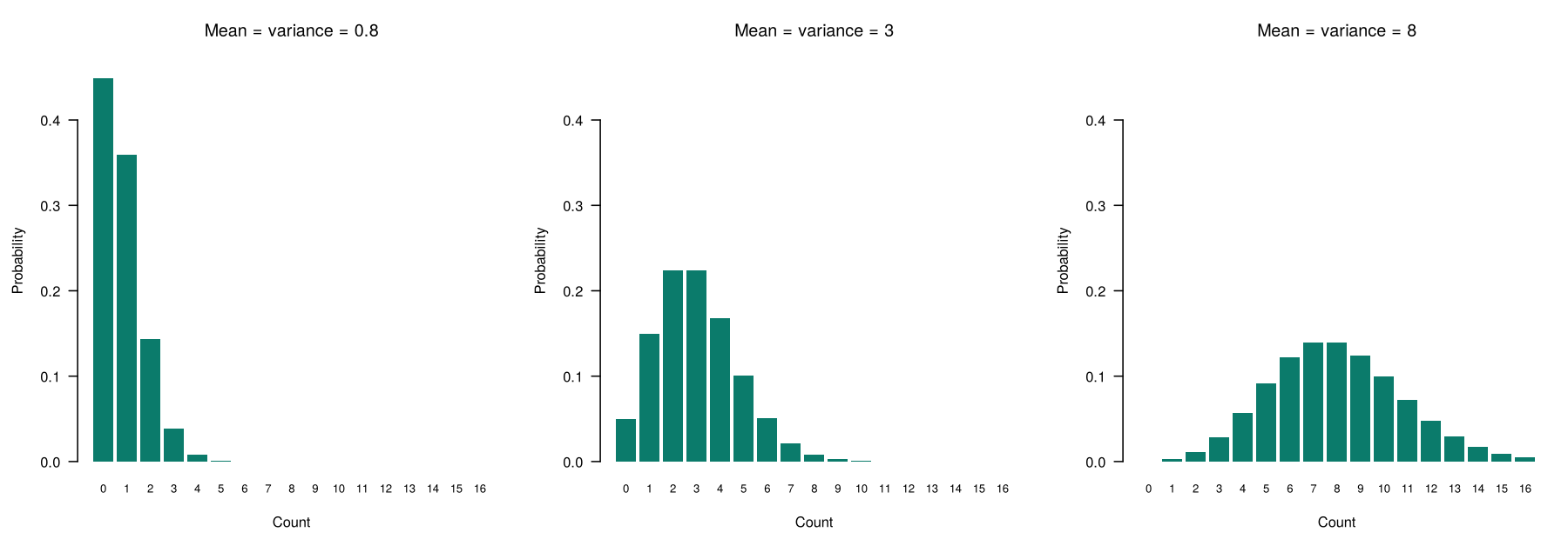
The Poisson distribution describes the number of events in a fixed period when events happen independently of one another at a constant average rate. It is named after the French mathematician Siméon-Denis Poisson. The whole distribution is defined by one number, its mean (written μ, the Greek letter mu), and its most important property is that its variance equals its mean. A Poisson count with a mean of 3 has a variance of 3, and a Poisson count with a mean of 0.8 has a variance of 0.8.
Figure 4.8 shows how the shape of the distribution changes as its mean increases.
The mean-equals-variance property is what makes the Poisson distribution simple, and it is also what most often goes wrong when it is applied to real health data. The checks later in this section are built around it.
Poisson regression, the subject of the next part, uses this distribution to model how the expected count changes with the predictors.
Poisson Regression
Poisson regression is the GLM with a Poisson distribution and a log link. The log of the expected count is set equal to the linear predictor.
Equation 4.5 gives the model for urgent care visits with age and smoking as predictors.
Because the predictors act by multiplication, the exponentiated coefficient eβ is a ratio of expected counts, called the incidence rate ratio (IRR). An IRR of 1 means no association, an IRR above 1 means more events, and an IRR below 1 means fewer events. In the PHAA data, the Poisson model gives an IRR for smoking of 1.44 (95% CI 1.19 to 1.73): smokers make about 44% more urgent care visits than non-smokers of the same age. The IRR for age is 1.013 per year (95% CI 1.007 to 1.018). Calculated from the unrounded coefficient, exp(10 × 0.01252) = 1.13 per ten years, or about 13% more visits for each decade of age.
Worked Example 4.4 calculates a crude rate ratio for smoking from the average numbers of visits in the two groups and compares it with the IRR from the model.
Worked Example 4.4: A Rate Ratio by Hand
Non-smokers (n = 662) made an average of 0.745 urgent care visits, and smokers (n = 133) made an average of 1.083. The crude ratio of these averages is 1.083 ÷ 0.745 = 1.45. The Poisson model's IRR of 1.44 is almost the same, because it also adjusts for age, which is only weakly related to smoking in these data.
The next part shows how the same model is adapted when the length of follow-up differs from person to person.
Different Follow-Up Times: The Offset
Every PHAA participant reported urgent care visits over the same 12 months, so their counts can be compared directly. Many studies instead follow people for different lengths of time, or count events in places with different population sizes. A person followed for ten years has more time to accumulate visits than a person followed for one year, and a city of a million people has more cases than a town of ten thousand. Poisson regression handles this with an offset: the log of each unit's follow-up time (or population size) is added to the model with its coefficient fixed at 1. The offset turns the model for counts into a model for rates, such as visits per person-year, which is why the exponentiated coefficients are called incidence rate ratios (Frome, 1983).
Worked code 4.1 fits a Poisson model with an offset to the PHAA follow-up file, in which the length of follow-up differs from person to person, and shows how its IRRs are then read as ratios of rates.
The PHAA follow-up file (phaa_followup.csv, used again in Lesson 5) records the number of GP visits each participant made during follow-up, which ranges from a few days to ten years (fu_years). Because follow-up time differs, the model needs offset(log(fu_years)).
fu <- read.csv("phaa_followup.csv")      # GP visits over 0 to 10 years of follow-up
fu$smoker <- factor(fu$smoker, levels = c("No", "Yes"))
gp <- glm(gp_visits ~ age + smoker + offset(log(fu_years)), data = fu, family = poisson)
round(exp(cbind(IRR = coef(gp), confint(gp))), 3)With the offset in place, the IRRs compare rates of GP visits per year of follow-up. Smokers have a GP visit rate 1.24 times that of non-smokers of the same age (95% CI 1.17 to 1.30), and the rate rises by about 1.8% for each year of age. The intercept (0.685) is the visit rate per year for a non-smoker aged 0 and is not interpreted. Without the offset, a person followed for ten years would appear to use far more care than a person followed for one year, simply because of the extra time.
An offset accounts for differences in follow-up time. The next part turns to the main check of a Poisson model, which concerns its assumption that the variance equals the mean.
Checking the Poisson Model: Overdispersion
The Poisson model assumes that the variance of the counts equals their mean, after the predictors are taken into account. When the variance is larger than the mean, the data are overdispersed. Overdispersion is common in health data, because people differ in ways the predictors do not capture: some people use health care much more than others of the same age and smoking status. Three checks reveal it.
Table 4.9 sets out the three checks, with the result of each for the PHAA data.
Table 4.9. Three checks for overdispersion in a Poisson model, with the results for urgent care visits in the PHAA data.
| Check | How it is calculated | Rule of thumb | PHAA result |
|---|---|---|---|
| Mean and variance of the counts | mean(y) and var(y) | A variance much larger than the mean is a warning sign (a first look only, because it ignores the predictors). | Mean 0.80, variance 1.76 |
| Dispersion ratio | Sum of squared Pearson residuals ÷ residual degrees of freedom | Close to 1 supports the Poisson model; clearly above 1 (for example, above about 1.5) signals overdispersion. | 2.05 |
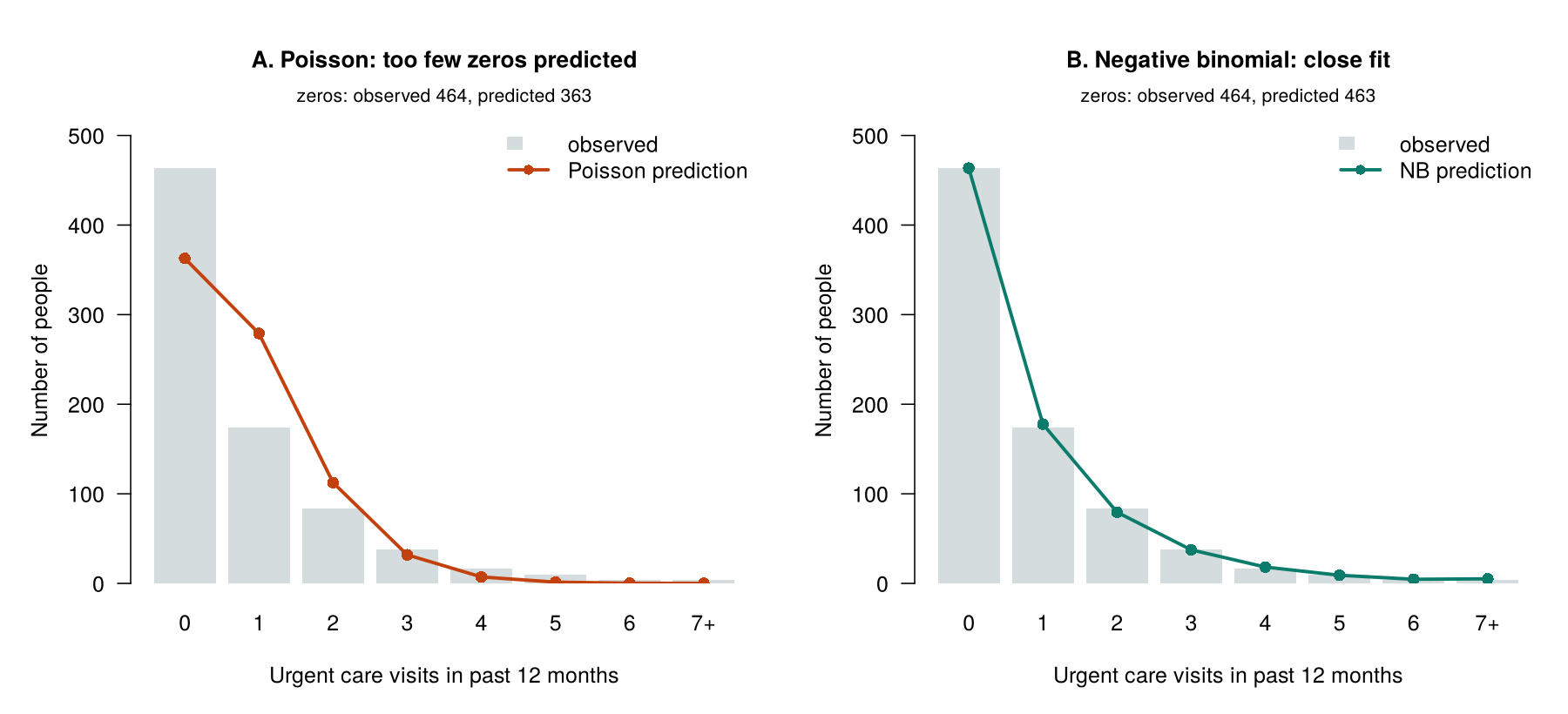
| Observed and expected zeros | sum(y == 0) and sum(dpois(0, fitted(model))) | The two numbers should be similar. | 464 observed, 363 expected |
All three checks point to overdispersion. The consequence is that the Poisson model is overconfident. Because it assumes a smaller variance than the data actually have, its standard errors are too small, its confidence intervals are too narrow and its p-values are too small. An analysis that ignored the problem could report an association as more certain than the data justify.
Figure 4.9 compares the observed numbers of people with each count of visits with the numbers expected by the Poisson model and by the negative binomial model introduced in the next part.
Box 4.7 describes a source of apparent overdispersion that should be ruled out before the Poisson model is replaced.
⚠ Box 4.7: Apparent overdispersion
Sometimes a Poisson model looks overdispersed because the model itself is incomplete: an important predictor is missing, or an offset for follow-up time has been left out. Before switching to a negative binomial model, it is worth asking whether the model includes the predictors and the offset that the study design calls for.
When the model includes the predictors and offset that it needs and the checks still show overdispersion, a model that allows the variance to exceed the mean is required. The next part introduces that model.
Negative Binomial Regression
Negative binomial regression keeps the log link and the IRR interpretation of Poisson regression and adds one extra parameter, θ (theta), that allows the variance to exceed the mean. The variance of a negative binomial count is μ + μ²/θ. A small θ means a lot of extra variation, and as θ becomes very large the second term shrinks toward zero and the model becomes a Poisson model (Hilbe, 2011). In R, the model is fitted with glm.nb() from the MASS package, and the output reports θ as Theta.
For the urgent care visits, θ is 0.77. The negative binomial model gives an IRR for smoking of 1.44 (95% CI 1.08 to 1.91), almost the same point estimate as the Poisson model. The confidence interval, however, is wider (it was 1.19 to 1.73 under the Poisson model), and the p-value rises from 0.0001 to 0.012. The IRR for age is 1.012 per year (95% CI 1.004 to 1.020). The associations remain, and the negative binomial model reports them with appropriate uncertainty.
Table 4.10 sets the results of the two models side by side.
Table 4.10. Results of the Poisson and negative binomial models for urgent care visits.
| Result | Poisson | Negative binomial |
|---|---|---|
| IRR for smoking (95% CI) | 1.44 (1.19 to 1.73) | 1.44 (1.08 to 1.91) |
| p-value for smoking | 0.0001 | 0.012 |
| IRR per year of age (95% CI) | 1.013 (1.007 to 1.018) | 1.012 (1.004 to 1.020) |
| AIC (lower is better) | 2154.9 | 1954.3 |
| Dispersion ratio | 2.05 | 0.99 |
| Expected zeros (464 observed) | 363 | 463 |
The comparison favours the negative binomial model on every check. The AIC (Akaike information criterion) measures how well a model fits the data, with a penalty for each parameter it estimates, and a lower value is better. A difference of about 10 points or more is usually taken as strong support for the model with the lower AIC (Burnham & Anderson, 2004), and here the difference is about 200 points. The dispersion ratio of the negative binomial model is 0.99, and it expects 463 zeros against the 464 observed.
The accordion below describes the models used when the counts contain many more zeros than even a negative binomial model expects.
In some data the number of zeros is much larger than even a negative binomial model expects. This often happens when part of the population cannot have the event at all, for example people who never use a particular service. Zero-inflated and hurdle models handle this situation by combining a model for "any events versus none" with a model for the number of events. They are fitted with the pscl package and are beyond the scope of this lesson. In the PHAA example, the negative binomial model already predicts the zeros well, so no further model is needed.
The two count models share most of their assumptions, and the next part sets them out together.
Assumptions and How to Check Them
Table 4.11 lists the assumptions of the Poisson and negative binomial models, whether each model requires them and how each is checked. The two models differ only in the assumption about the variance.
Table 4.11. The assumptions of the Poisson and negative binomial models and how each is checked.
| Assumption | Poisson | Negative binomial | How to check it |
|---|---|---|---|
| The outcome is a count (whole numbers of 0 or more) | Required | Required | table(outcome) or summary(outcome) |
| Independent observations | Required | Required | Judged from the study design |
| Each predictor multiplies the expected count (log link) | Required | Required | Built into the model; for a continuous predictor, a squared term can test for curvature |
| Different follow-up times are accounted for | Offset needed | Offset needed | offset(log(time)) in the formula |
| The variance equals the mean | Required | Relaxed: variance may be larger | Dispersion ratio; observed versus expected zeros; AIC comparison |
With the count models complete, the last part of this section draws the four sections of the lesson together.
Bringing the Lesson Together
The four sections of this lesson apply the same approach to five types of outcome. The type of the outcome is identified first, and it points to a model. The model is fitted with the same linear predictor (here, age and smoking), its exponentiated coefficients are read as the ratio that its link function implies, and its own assumptions are checked before the results are reported.
Table 4.12 summarises the five PHAA examples, with the model, the effect of smoking and the main check for each.
Table 4.12. The five types of outcome in the PHAA examples, with the model and R function, the effect of smoking (95% CI) and the main check for each.
| Outcome type (PHAA example) | Model and R function | Effect of smoking | Main check |
|---|---|---|---|
| Continuous (systolic blood pressure) | Linear, lm() | +6.06 mmHg (4.33 to 7.79) | Residual plots |
| Binary (hypertension) | Logistic, glm(family = binomial) | OR 2.65 (1.04 to 6.30) | Events per predictor |
| Ordinal (self-rated health) | Ordinal logistic, polr() | OR 0.50 for a higher category (0.36 to 0.70) | Brant test |
| Nominal (usual place of care) | Multinomial logistic, multinom() | RRR 3.01 for emergency department versus family doctor (1.57 to 5.75) | People per category; IIA |
| Count (urgent care visits) | Negative binomial, glm.nb() | IRR 1.44 (1.08 to 1.91) | Dispersion ratio, AIC, zeros |
The card below links to a narrated walkthrough of count models in R. Activity 4.5 fits the Poisson model for urgent care visits and runs the overdispersion checks in Table 4.9, and Activity 4.6 fits the negative binomial model and reproduces the comparison in Table 4.10. A knowledge check and a reflection close the section, and the final page of the lesson gathers its key takeaways.
Narrated R walkthrough: Poisson and Negative Binomial Regression in R
This walkthrough models a count outcome. It compares the mean and the variance of the counts, fits a Poisson regression and reads its rate ratios, checks for overdispersion, fits a negative binomial regression and compares the two models.
Open the Poisson and Negative Binomial Regression in R walkthroughThis activity fits a Poisson regression for urgent care visits and checks it for overdispersion. Activity 4.6 continues from this one, so both are best run in the same R session.
library(MASS)    # glm.nb() fits the negative binomial model (next activity)
phaa <- read.csv("phaa_outcomes.csv")   # file must be in the working directory
phaa <- na.omit(phaa)                   # keep the 795 people with no missing values
phaa$smoker <- factor(phaa$smoker, levels = c("No", "Yes"))   # "No" = reference
table(phaa$urgent_visits)    # how many people had 0, 1, 2, ... visits
mean(phaa$urgent_visits)     # the average count
var(phaa$urgent_visits) # the variance (spread) of the countsThe table shows the shape of a typical count: 464 people with no visits, 174 with one visit and a long tail up to 12 visits. The mean (0.80) and the variance (1.76) give a first warning, because a Poisson count would have a variance close to its mean.
pois <- glm(urgent_visits ~ age + smoker, data = phaa, family = poisson)
summary(pois)
exp(cbind(IRR = coef(pois), confint(pois))) # incidence rate ratios with 95% CIsReading the output. The Estimate column is on the log scale, so the last line exponentiates it to give incidence rate ratios. The IRR for smoking is 1.44 (95% CI 1.19 to 1.73): smokers make about 44% more urgent care visits than non-smokers of the same age. The IRR for age is 1.013 per year (95% CI 1.007 to 1.018). The line (Dispersion parameter for poisson family taken to be 1) is a reminder that the model assumes that the variance equals the mean.
# Check 1: the dispersion ratio is close to 1 when the Poisson model fits
sum(residuals(pois, type = "pearson")^2) / df.residual(pois)
# Check 2: compare the zeros we observed with the zeros the model expects
sum(phaa$urgent_visits == 0)
sum(dpois(0, fitted(pois)))The dispersion ratio is 2.05, about twice the value of 1 that a Poisson model assumes. The data contain 464 people with zero visits, but the Poisson model expects only about 363. Both checks show overdispersion, so the confidence intervals from this model are too narrow and its p-values are too small.
R Reflect on what you just ran
Use the questions below to interpret the output you produced. Look at your console output before answering.
1. Report the incidence rate ratio for smokerYes from the Poisson model with its 95% confidence interval, and explain it in one sentence.
2. Report the dispersion ratio and the observed and expected numbers of zeros. What do they tell you about the Poisson model?
3. A colleague argues that the overdispersion does not matter, because the IRR for smoking is clearly above 1. Explain why the overdispersion still matters for the conclusions.
This activity continues from Activity 4.5 above. It uses the phaa data frame and the pois model created there, and the glm.nb() function from the MASS package loaded at its start.
nb <- glm.nb(urgent_visits ~ age + smoker, data = phaa)
summary(nb)
exp(cbind(IRR = coef(nb), confint(nb))) # incidence rate ratios with 95% CIsReading the output. The coefficients look much like those of the Poisson model, but their standard errors are larger (0.145 for smoking, compared with 0.095). Theta (0.77) is the extra parameter that lets the variance exceed the mean. The IRR for smoking is 1.44 (95% CI 1.08 to 1.91), and its p-value is 0.012, compared with 0.0001 under the Poisson model.
AIC(pois, nb)                                               # lower AIC = better fit
sum(residuals(nb, type = "pearson")^2) / df.residual(nb)    # dispersion ratio for NB
sum(dnbinom(0, mu = fitted(nb), size = nb$theta)) # zeros expected by NBThe AIC is 1954.3 for the negative binomial model and 2154.9 for the Poisson model, a difference of about 200 points in favour of the negative binomial model. Its dispersion ratio is 0.99, and it expects about 463 zeros against the 464 observed. On all three checks, the negative binomial model fits these data and the Poisson model does not.
R Reflect on what you just ran
Use the questions below to interpret the output you produced. Look at your console output before answering.
1. Compare the IRR for smoking and its 95% confidence interval from the Poisson and negative binomial models. What changed, what stayed the same, and why?
2. Use the AIC values and the dispersion ratio to justify which model you would report.
3. Write one sentence that reports the negative binomial result for smoking as it might appear in the results section of a paper.
1. What is the special property of the Poisson distribution that a Poisson regression assumes?
2. A Poisson regression of the number of falls gives an IRR of 0.75 for a balance-training program. What does this mean?
3. When is an offset needed in a Poisson or negative binomial model?
4. A Poisson model has a dispersion ratio of 2.4. What is the most appropriate next step?
5. Compared with a Poisson model of overdispersed counts, a negative binomial model usually gives:
✎ Reflection
This section showed that counts (whole numbers of 0 or more, usually with many zeros) are modelled with Poisson regression, which uses a log link so that exponentiated coefficients are incidence rate ratios (IRRs). Poisson regression assumes that the variance of the counts equals their mean, which is checked with the dispersion ratio (close to 1 when the model fits) and by comparing observed and expected zeros. When the counts are overdispersed, negative binomial regression adds a parameter (theta) that lets the variance exceed the mean, and the two models are compared with the AIC. An offset, the log of follow-up time, is added when people are observed for different lengths of time. A city health unit records, for each of its 40 neighbourhoods, the number of opioid overdose calls to paramedics over one year, along with each neighbourhood's population and median income. Describe how you would model the number of calls in relation to median income: which model you would start with, why an offset is needed and what it would be, which checks you would run on the first model, what you would do if the checks failed, and how you would interpret an IRR of 0.80 for each $10,000 increase in median income.
Lesson 4: Final Assessment
Bringing It All Together
This lesson presented one regression model for each common type of outcome. Section 1 sorted variables into numeric (continuous or discrete) and categorical (binary, ordinal or nominal) types, reviewed the four assumptions of linear regression (linearity, independence, normality and equal variance of the residuals) and the plots that check them, and introduced the generalized linear model, which keeps the linear predictor and changes the distribution and the link function. It also reviewed logistic regression for binary outcomes and its requirement of enough events per predictor.
Section 2 fitted ordinal logistic regression to self-rated health. The model fits every at-or-above split of the outcome at once and gives each predictor one odds ratio for being in a higher category, an assumption that the Brant test checks. Section 3 fitted multinomial logistic regression to usual place of care. The model compares each category with a reference category, reports relative risk ratios for each comparison, and is often clearest when presented as predicted probabilities. Section 4 fitted Poisson regression to urgent care visits, found that the counts were overdispersed (a dispersion ratio of 2.05 and too few expected zeros), and fitted a negative binomial model that matched the data and gave wider confidence intervals that reflect the extra variation in the counts.
Across the lesson, the same two predictors were used with five different outcomes, and the same steps were followed each time: the outcome type was identified, the matching model was fitted, the exponentiated coefficients were read as the ratio that the link function implies, and the model's own assumptions were checked before the results were reported. The final assessment asks for these steps to be applied to new outcomes. The next lesson, Modelling Dependent Data, takes up the one assumption that every model in this lesson shares and that none of them can check from its own output: the independence of the observations.
Key Takeaways from this lesson
- The type of the outcome (continuous, count, binary, ordinal or nominal) decides which model is used, and it is identified before any model is fitted.
- Linear regression assumes linearity, independence, normality of the residuals and equal variance, and all except independence are checked with
plot(model). - A generalized linear model has a distribution, a linear predictor and a link function, and the link decides whether an exponentiated coefficient is an odds ratio, a relative risk ratio or an incidence rate ratio.
- Ordinal logistic regression gives one odds ratio per predictor for being in a higher category, and the Brant test checks that this odds ratio is the same at every split.
- Multinomial logistic regression compares each category with a reference category, needs enough people in every category, and is often best presented with predicted probabilities.
- Poisson regression assumes that the variance of the counts equals their mean, and a dispersion ratio well above 1 signals overdispersion that makes its confidence intervals too narrow.
- Negative binomial regression allows the variance to exceed the mean, keeps the incidence rate ratio interpretation, and is preferred when it has a clearly lower AIC.
The final assessment covers all four sections. All 15 questions must be answered correctly (100%), and the final reflection completed, to finish the lesson.
Reflection
A study follows 1,200 adults aged 65 and older who live at home. For each person it records three outcomes over one year: the number of falls (most people have none and a few have many); fear of falling, rated as not afraid, somewhat afraid or very afraid; and the main type of help the person receives at home (none, a family member, paid home care, or a community program). The predictors are age, gender and whether the person lives alone. This lesson matched outcome types to models: linear regression for continuous outcomes (checked with residual plots), logistic regression for binary outcomes (checked by counting events per predictor), ordinal logistic regression for ordered categories (fitted with polr() and checked with the Brant test), multinomial logistic regression for unordered categories (fitted with multinom(), using a reference category and checked for enough people in each category and for categories that are not close substitutes), and Poisson or negative binomial regression for counts (fitted with glm(family = poisson) or glm.nb() and compared with the dispersion ratio and the AIC). For each of the three outcomes, state its type, the model and R function you would use, what the exponentiated coefficients would be called and how you would explain one of them, and the main assumption you would check.
glm(falls ~ age + gender + lives_alone, family = poisson); everyone was followed for one year, so no offset is needed. Its exponentiated coefficients are incidence rate ratios: an IRR of 1.5 for living alone would mean that people living alone have 1.5 times as many falls as people of the same age and gender who live with others. With many zeros and a few people with many falls, overdispersion is likely, so I would check the dispersion ratio and the observed versus expected zeros, and if the ratio were clearly above 1 I would fit glm.nb() and compare the AIC values. Fear of falling is ordinal (not afraid, somewhat afraid, very afraid), so I would use ordinal logistic regression with polr(), after setting the levels in order with factor(..., ordered = TRUE). Its exponentiated coefficients are odds ratios for being in a higher (more afraid) category: an odds ratio of 1.3 per five years of age would mean 1.3 times the odds of being in a more afraid category at either split. The main check is the proportional-odds assumption with brant(), with a multinomial model as a fallback if it failed. The main type of home help is nominal, so I would use multinomial logistic regression with multinom(), with "none" as the reference category, which gives three comparisons. Its exponentiated coefficients are relative risk ratios: an RRR of 2.0 for living alone in the paid home care comparison would mean that the ratio of paid home care to no help is twice as high for people living alone. I would check that every category has enough people within each predictor group with table(), and consider whether any two categories (for example, paid home care and a community program) are close substitutes, which would weaken the IIA assumption. For all three outcomes, independence holds if each person is counted once.Minimum 20 characters required.
Final Knowledge Assessment
1. A study records the number of prescriptions each person fills in a year. Which model is the natural starting point?
2. Which model suits the outcome "highest level of education completed" (less than high school, high school, college, university)?
3. Which model suits the outcome "blood type" (A, B, AB, O)?
4. In the residual plots of a linear regression, the spread of the residuals widens like a funnel from left to right. Which assumption is in doubt?
5. Which assumption of linear regression is judged from the study design and cannot be checked with plot(model)?
6. Which description fits logistic regression as a generalized linear model?
7. The exponentiated coefficients of a multinomial logistic regression are called:
8. In a polr() model of self-rated health (ordered Poor to Excellent), the odds ratio for smoking is 0.50. Which statement is correct?
polr(), an odds ratio below 1 means lower odds of being in a higher category, and the proportional-odds model applies the same odds ratio at every split.9. The Brant test for an ordinal model gives an omnibus p-value of 0.62 and p-values above 0.30 for every predictor. What should be concluded?
10. A multinomial model is fitted to an outcome with three categories. How many sets of coefficients (comparisons) does it estimate?
11. For any one person, the predicted probabilities from a multinomial model across all of the outcome categories:
12. A Poisson regression of emergency visits gives an IRR of 1.30 for people without a family doctor. What does this mean?
13. A Poisson model has a dispersion ratio of 1.03 and expects about as many zeros as are observed. What should be concluded?
14. Why is an offset of log(follow-up time) added to a Poisson model?
15. A Poisson model and a negative binomial model fitted to the same counts have AIC values of 1500 and 1420. Which statement is correct?
✦ Before submitting: pass every section knowledge check (100%) and complete every reflection.