This glossary collects the key concepts, methods and people in this lesson. It can be used as a reference while working through the material or as a review before assessments. Typing in the search box filters the entries.

Lesson 5 · Section 1

Recognising Dependent Data

When observations share a clinic, a household or a person, they are no longer independent of one another.

Two forms

Clustered data and repeated measures

Clustered data

People are grouped inside larger units, such as patients in clinics, students in schools or residents in neighbourhoods.

Repeated measures

The same person is measured several times, so each person's measurements form a cluster.

In both forms, observations from the same cluster tend to be more alike than observations from different clusters.

Why it matters

Ignoring dependence makes a model overconfident

• The model counts every observation as a separate piece of information.
• Its standard errors are too small, its confidence intervals too narrow and its p-values too small.
• The problem is largest for predictors that describe the cluster, such as an urban or rural clinic.

Running example

966 patients in 30 clinics

Measuring clustering

The intracluster correlation coefficient (ICC)

Intracluster correlation coefficient

\[ \text{ICC} = \frac{\color{#C2410C}{\sigma^2_{\text{between}}}}{\color{#C2410C}{\sigma^2_{\text{between}}} + \color{#0B7B6B}{\sigma^2_{\text{within}}}} \]

σ²_between variance between cluster averages σ²_within variance among people in the same cluster

The ICC is also the correlation between the outcomes of two people in the same cluster.

What the ICC looks like

Three levels of clustering

ICC in the clinic data

About 17.5% of the variation lies between clinics

22.1

variance between clinics

104.3

variance within clinics

0.175

ICC = 22.1 ÷ (22.1 + 104.3)

ICCs for clinics, schools and neighbourhoods are often between 0.01 and 0.1, so 0.175 indicates strong clustering.

Design effect

From 966 patients to about 150 independent people

Design effect and effective sample size

\[ \text{DEFF} = 1 + (\color{#0B7B6B}{\bar m} - 1) \times \color{#C2410C}{\text{ICC}} \qquad n_{\text{eff}} = \frac{n}{\text{DEFF}} \]

m̄ average cluster size (32.2) ICC intracluster correlation coefficient (0.175)

6.45

design effect ≈ 1 + 31.2 × 0.175

150

effective sample size = 966 ÷ 6.45

What goes wrong

The same difference, with and without allowing for clinics

Which predictors are affected?

Cluster-level predictors lose the most precision

Cluster-level predictors

These take the same value for everyone in a cluster, such as an urban clinic or a school assigned to one trial arm. Their standard errors grow the most.

Person-level predictors

These vary within each cluster, such as age or smoking. Their standard errors change little and can even shrink.

Two families of methods

Mixed models and GEE

Method	What it does	R function
Linear mixed model	Gives each cluster its own baseline (a random intercept) for a continuous outcome	lme4::lmer()
Generalized linear mixed model (GLMM)	Adds a random intercept to a logistic or Poisson model	lme4::glmer()
Generalized estimating equations (GEE)	Fits a regression for the whole population, with standard errors that allow for clustering	geepack::geeglm()

Carry forward

What to take into the next section

• Observations are dependent when they share a cluster, such as a clinic or a person measured several times.
• The ICC measures how alike observations in a cluster are, and the design effect shows the information lost.
• Ignoring dependence makes a model overconfident, and mixed models and GEE are the standard remedies.

Introduction and Overview

Every regression model in Lessons 3 and 4 assumed that the observations are independent, so that one person's outcome carries no information about another person's outcome. This lesson deals with data in which that assumption fails. Observations are dependent when they share something, such as patients attending the same clinic or the same person measured at several visits. This first section explains how to recognise dependent data, how to measure the strength of the dependence with the intracluster correlation coefficient (ICC) and the design effect, and what goes wrong when the dependence is ignored. The later sections fit models that allow for it.

What Are Dependent Data?

Data are dependent when observations can be grouped into clusters whose members are more alike than members of different clusters. Two forms are common in public health. In clustered data, people are grouped inside larger units: patients in clinics, students in schools, residents in neighbourhoods, or workers in workplaces. People in the same cluster share a setting, staff, policies and local conditions, so their outcomes tend to be similar. In repeated measures (also called longitudinal data), the same person is measured more than once, and each person's measurements form a cluster. Clusters can also be nested inside one another, such as patients within doctors within clinics, which this lesson mentions only briefly.

Table 5.1 gives four examples of studies that produce dependent data, with the cluster, the observation and the reason why observations in the same cluster are alike.

Table 5.1. Examples of clustered data and repeated measures in public health studies.

The three flip cards below define the cluster, independence and the effective sample size, terms that the rest of the lesson uses repeatedly.

Dependent data therefore arise whenever a study samples people in groups or measures the same people repeatedly, and every method in this lesson needs the variable that identifies the clusters. The next part explains why this grouping matters for a regression model.

Why Dependence Matters

A regression model that assumes independence treats every observation as a separate piece of information. When observations in a cluster are alike, part of what each one says has already been said by the others, so the model overstates how much information it has. The point estimates are often similar, but the standard errors are too small, the confidence intervals too narrow and the p-values too small. In practice, this means that an analysis that ignores clustering can report a statistically significant association that the data do not support (Dohoo, Martin & Stryhn, 2012, Chapter 20).

The clinic data introduced next show how large this effect can be.

The Clinic Data

The first three sections of this lesson use phaa_clinics.csv, a simulated dataset of 966 patients attending 30 primary care clinics, with between 18 and 45 patients per clinic (32.2 on average). It records each patient's age, gender (female = 1 for women), smoking status, BMI, systolic blood pressure (sbp) and whether they were referred to a specialist (referred = 1). Two variables describe the clinic itself: clinic_urban (20 urban and 10 rural clinics) and clinic_size.

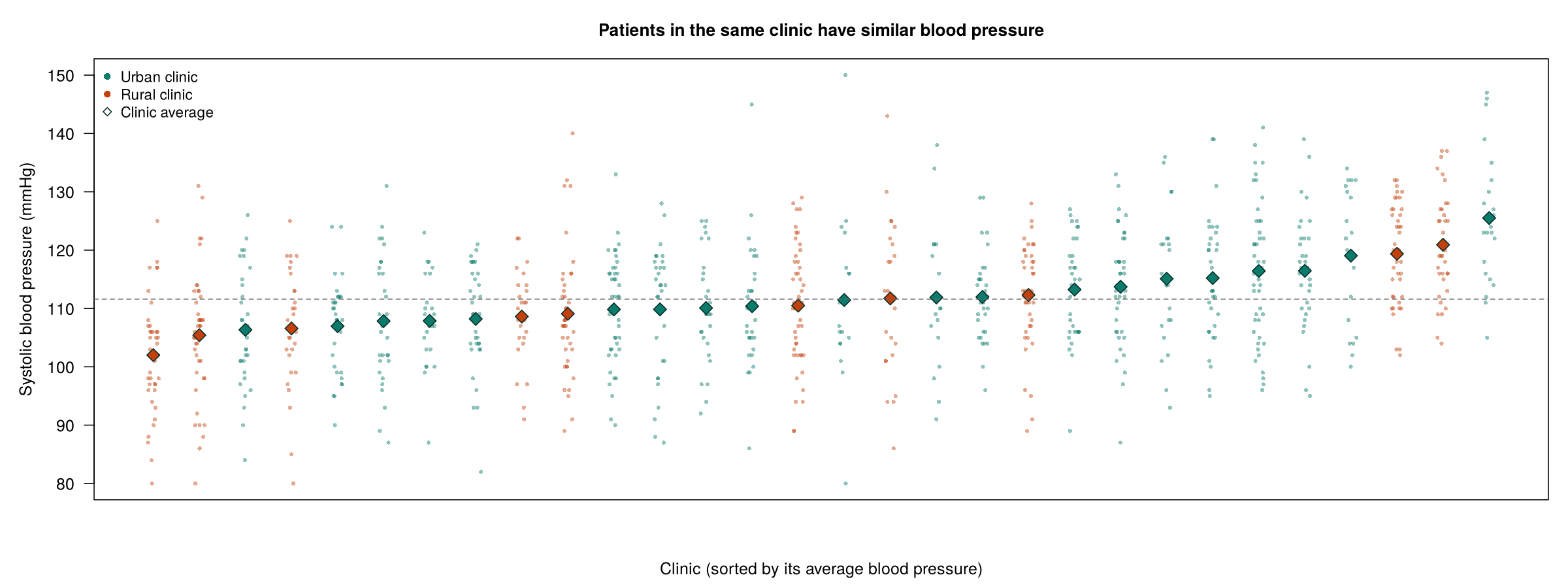
Figure 5.1 plots the systolic blood pressure of every patient by clinic, so that the differences between clinic averages can be seen before any model is fitted.

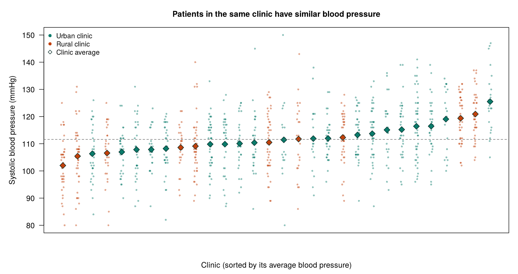
Figure 5.1 shows that a patient’s blood pressure depends partly on the clinic the patient attends. The intracluster correlation coefficient, introduced next, measures how much of the variation in blood pressure lies between clinics.

Measuring Clustering: The Intracluster Correlation Coefficient

The intracluster correlation coefficient (ICC) measures how alike observations in the same cluster are. It divides the total variance of the outcome into a part between clusters (how much the cluster averages differ) and a part within clusters (how much people in the same cluster differ from one another), and it is the share of the total that lies between clusters. Equation 5.1 expresses this share as a ratio of the two variances.

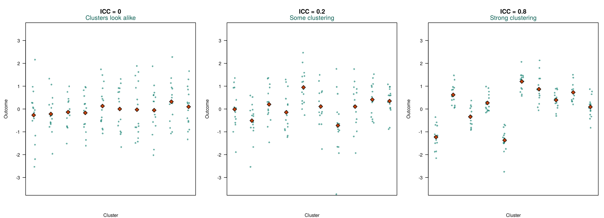
The ICC can also be read as the correlation between the outcomes of two people chosen from the same cluster. Lesson 7 uses a statistic of the same form, the intraclass correlation coefficient, for a different application: measuring the reliability of a score across occasions or raters. Figure 5.2 shows simulated clusters with three values of the ICC.

Worked Example 5.1 applies Equation 5.1 to the clinic data, using the two variances that Activity 5.1 estimates at the end of this section.

The ICC of 0.175 measures the strength of the clustering in the clinic data. The next part converts it into a loss of information with the design effect and the effective sample size.

The Design Effect and the Effective Sample Size

The design effect (DEFF) expresses the ICC as a loss of information. It depends on both the ICC and the average cluster size. Equation 5.2 gives the design effect and the effective sample size that follows from it.

For the clinic data, DEFF = 1 + (32.2 − 1) × 0.1748 = 6.45 (using the unrounded ICC), and the effective sample size is 966 ÷ 6.45 = 150. For questions about clinic characteristics, the 966 clustered patients therefore carry about as much information as 150 independent people. The formula also shows why cluster size matters: with 32 people per cluster, even an ICC of 0.05 gives a design effect of 1 + 31 × 0.05 = 2.55, which reduces the effective sample size by more than half. Design effects are also used when planning studies, to inflate the sample size needed for a cluster-sampled survey or a cluster-randomized trial. Students who took HSCI 230 or HSCI 341 met this formula in HSCI 230 Lesson 5, Section 6, and HSCI 341 Lesson 2, Section 5, where it inflates the sample size of a planned study; this section uses the same formula to describe the information lost in an analysis.

The effective sample size of about 150 summarises how much information the clustering removes from the clinic data for questions about clinic characteristics. The next part shows how this loss appears in a regression model that ignores the clinics.

What Goes Wrong When Clustering Is Ignored

The question of whether patients in urban clinics have higher blood pressure than patients in rural clinics shows the problem directly. An ordinary linear regression with lm() treats the 966 patients as independent. A linear mixed model with lmer() gives each clinic its own baseline, as Section 2 explains.

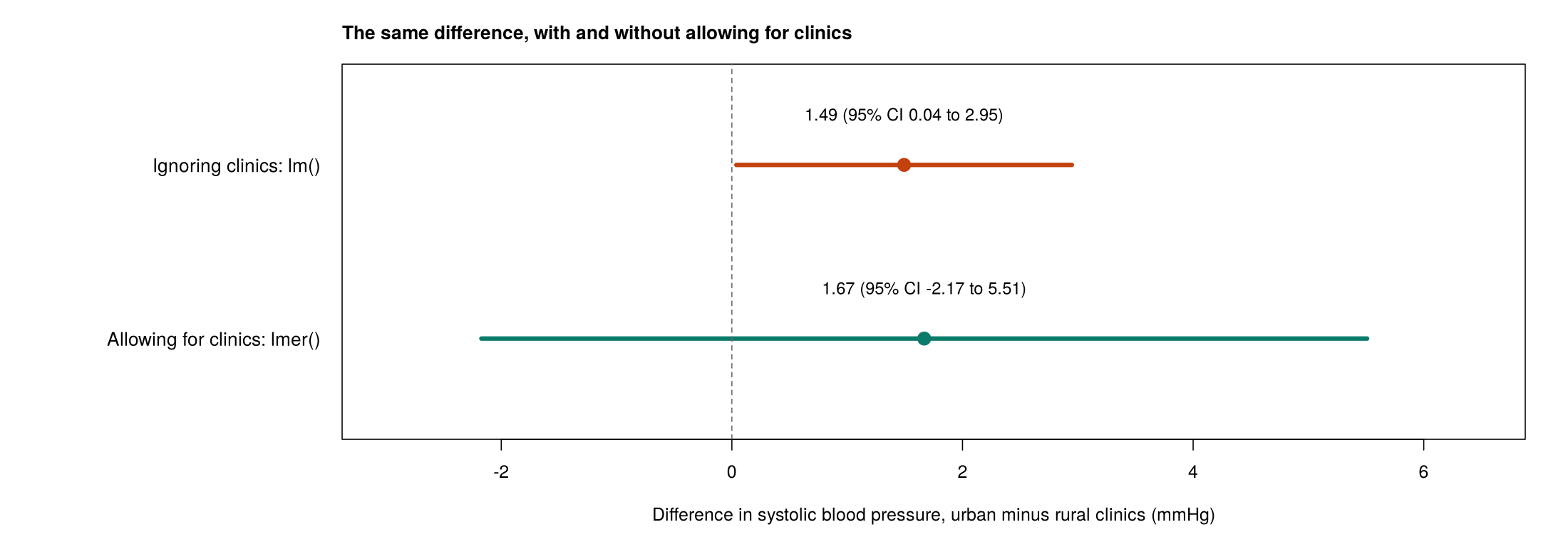
Figure 5.3 compares the two estimates of the urban minus rural difference with their 95% confidence intervals, and Table 5.2 gives the estimates, standard errors and p-values from the two models.

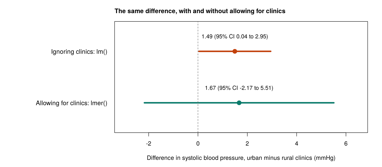
Table 5.2. The urban minus rural difference in systolic blood pressure from an ordinary regression and a linear mixed model.

The ordinary regression suggests a statistically significant difference, and the mixed model shows that the data cannot distinguish urban from rural clinics. The standard error rises from 0.74 to 1.96 because clinic_urban is a cluster-level predictor: it takes one value per clinic, so the 966 patients supply only 30 independent values of it. A person-level predictor such as smoking varies among patients within each clinic, and its standard error changes little when clustering is taken into account (in the Section 2 model, which adds age, gender and smoking, it falls from 0.79 to 0.70, and Section 3 shows a similar pattern for referrals). When a predictor varies within clusters, allowing for clustering can make its estimate more precise, because the model can compare people within the same clinic.

Box 5.1 adds a caution about how this problem is detected in practice.

A clustered dataset therefore needs a method that allows for the clustering, and the next part introduces the two families of methods that the lesson uses.

Methods for Dependent Data

Two families of methods are used throughout this lesson. Mixed models add a random effect for each cluster and estimate how much the clusters vary; GEE fits a regression with no cluster effects, so the results describe the population as a whole, and calculates standard errors that allow for the correlation within clusters. Both need a variable that identifies the clusters. Simpler approaches also exist, such as analysing cluster averages or adding a separate indicator variable for every cluster, but they lose information or cannot estimate the effects of cluster-level predictors, and this lesson does not use them.

Table 5.3 lists the three models that the lesson fits, with the outcomes they handle, the R function for each and the sections in which they are used.

Table 5.3. Methods for dependent data used in this lesson.

This section has established that dependence arises from the design of a study, that the ICC and the design effect measure its strength, and that ignoring it understates the uncertainty for cluster-level predictors. The narrated R walkthrough below demonstrates all of the methods in Table 5.3 on the lesson’s two datasets. Activity 5.1 then reproduces the main results of this section, from the ICC to the comparison in Table 5.2, before the knowledge check for the section.

# install.packages(c("lme4", "lmerTest", "geepack"))   # run once, if not yet installed
library(lmerTest)    # loads lme4 (for lmer()) and adds p-values
clinics <- read.csv("phaa_clinics.csv")   # file must be in the working directory
clinics$clinic_id <- factor(clinics$clinic_id)
clinics$smoker <- factor(clinics$smoker, levels = c("No", "Yes"))
clinics$clinic_urban <- factor(clinics$clinic_urban, levels = c("rural", "urban"))
nlevels(clinics$clinic_id)                        # how many clinics?
summary(as.vector(table(clinics$clinic_id)))      # patients per clinic

m0 <- lmer(sbp ~ 1 + (1 | clinic_id), data = clinics)   # a model with clinics only
vc <- as.data.frame(VarCorr(m0))
vc[, c("grp", "vcov")]                    # variance between clinics and within clinics
icc <- vc$vcov[1] / sum(vc$vcov)          # intracluster correlation coefficient
icc

m_bar <- mean(table(clinics$clinic_id))   # average clinic size
deff  <- 1 + (m_bar - 1) * icc             # design effect
deff
nrow(clinics) / deff                       # effective sample size

naive <- lm(sbp ~ clinic_urban, data = clinics)                     # ignores clinics
mixed <- lmer(sbp ~ clinic_urban + (1 | clinic_id), data = clinics)  # allows for clinics
summary(naive)$coefficients
summary(mixed)$coefficients

Lesson 5 · Section 2

Linear Mixed Models

A model for a continuous outcome that gives each cluster its own baseline.

The idea

Each clinic gets its own baseline

Random-intercept linear mixed model

\[ \text{SBP}_{ij} = \color{#6D28D9}{\beta_0} + \color{#C2410C}{u_j} + \color{#1D4ED8}{\beta_1}\,\text{age}_{ij} + \dots + \color{#0B7B6B}{\varepsilon_{ij}}, \qquad \color{#C2410C}{u_j} \sim N(0, \sigma^2_u) \]

β₀ overall intercept u_j shift for clinic j (random effect) β₁, … fixed effects, read as in Lesson 4 ε_ij difference for patient i within the clinic

The model estimates one variance, σ²_u, that describes how much the clinic baselines differ.

Two kinds of effects

Fixed effects and random effects

Fixed effects

These are the coefficients for the predictors, read as differences in average blood pressure, as in Lesson 4.

Random effects

These are the clinic shifts, summarised by their variance or standard deviation.

lmer(sbp ~ age + female + smoker + clinic_urban + (1 | clinic_id), data = clinics)

The term (1 | clinic_id) asks for a random intercept for each clinic.

Reading the output

Fixed effects from lmer()

Predictor	Estimate (mmHg)	95% CI	p-value
Age (per year)	0.41	0.37 to 0.45	< 0.001
Female	−2.80	−3.88 to −1.73	< 0.001
Smoker	5.00	3.63 to 6.37	< 0.001
Urban clinic	1.85	−1.85 to 5.54	0.34

The random effects show a standard deviation of 4.6 mmHg between clinic baselines and 8.3 mmHg among patients within a clinic.

The clinic effects

Clinics differ by several mmHg, after adjustment

Interpretation

What a fixed effect means

• The smoking coefficient compares a smoker and a non-smoker of the same age and gender in the same clinic.
• For a continuous outcome, this is also the average difference in the whole population.
• The main gain from the mixed model is a standard error that reflects the clustering.

Model checking

Three plots check most of the assumptions

Further checks

Enough clusters, and no singular fit

Assumption	How to check it	This example
Linearity and equal variance	Residuals versus fitted values	Acceptable
Normal residuals	Q-Q plot of residuals	Acceptable
Normal clinic effects	Q-Q plot of the random effects	Three high clinics
Enough clusters (about 20 to 30)	nlevels(clinic_id)	30 clinics
Clinic variance estimated	isSingular(model)	FALSE

Going further

Random slopes

Random intercept

Clinic baselines differ, and each predictor has the same effect in every clinic.

(1 | clinic_id)

Random slope

The effect of a predictor, such as age, is also allowed to differ between clinics.

(age | clinic_id)

Random slopes need more clusters and often trigger warnings with small samples.

Carry forward

What to take into the next section

• A random intercept gives each cluster its own baseline, summarised by one variance.
• Fixed effects are read as in an ordinary regression, and random effects describe the clusters.
• The checks are residual plots, a Q-Q plot of cluster effects, the number of clusters and the singular-fit warning.

Introduction and Overview

This section presents the linear mixed model, the standard model for a continuous outcome when observations are clustered. It continues with systolic blood pressure in the 30 clinics of phaa_clinics.csv, now with four predictors: age, gender, smoking and whether the clinic is urban. The section explains the random intercept, shows how to read the fixed and random parts of the R output, lists the checks that a mixed model needs, and describes random slopes briefly.

The Random-Intercept Model

An ordinary linear regression has a single intercept. A random-intercept model gives each cluster its own intercept, made up of the overall intercept plus a cluster-specific shift. The shifts are treated as a random sample from a normal distribution with mean 0, and the model estimates the variance of that distribution, which describes how much the clusters differ (Laird & Ware, 1982). Equation 5.3 writes the model for systolic blood pressure in the clinic data.

The name "mixed" refers to the two kinds of effects in the model. The fixed effects (β₀ to β₄) are the coefficients for the predictors, read as differences in average blood pressure, as in Lesson 4. The random effects (u_j) are the clinic shifts, summarised by their variance. Summarising the 30 clinics with one variance lets the model estimate the effect of a clinic-level predictor such as clinic_urban.

The three flip cards below restate the random intercept, the fixed effects and the variance components, with the lmer() notation for the random intercept.

With the parts of the model defined, the next part reads them from the R output for the clinic data.

Reading the Output

Activity 5.2 below fits the model with lmer() after loading the lmerTest package, which adds p-values to the fixed effects. The output has two main blocks. Table 5.4 summarises the fixed-effects block, with a 95% confidence interval and an interpretation for each predictor.

Table 5.4. Fixed effects from the random-intercept model for systolic blood pressure.

Each estimate holds the other predictors constant. The df column of the output shows about 937 degrees of freedom for the patient-level predictors and about 28 for urban clinics, because the information about a clinic-level predictor comes from the 30 clinics.

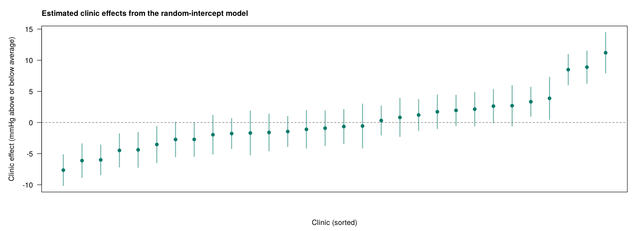
The random effects block reports a clinic variance of 21.57 (standard deviation 4.64 mmHg) and a residual variance of 68.94 (standard deviation 8.30 mmHg). The adjusted ICC is 21.57 ÷ (21.57 + 68.94) = 0.24. It is larger than the ICC of 0.175 from the model with no predictors, because age, gender and smoking explain much of the variation among patients within clinics but little of the variation between clinics. Figure 5.4 shows the estimated shifts of the 30 clinic baselines, which the clinic variance summarises.

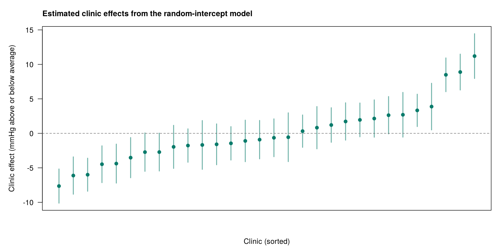
Worked Example 5.2 uses the intercept and the fixed effects of the model to predict blood pressure for two patients, and shows how a clinic shift such as those in Figure 5.4 changes the predictions.

These interpretations depend on the model being appropriate for the data, so the next part sets out the assumptions of a linear mixed model and how to check them.

Assumptions and How to Check Them

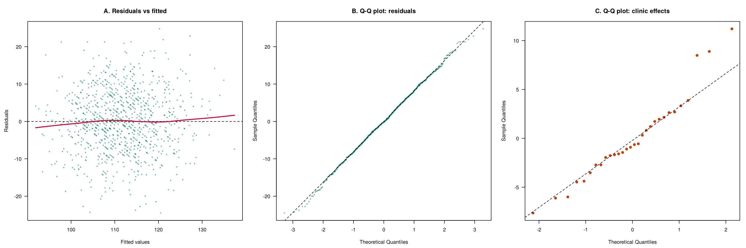
A linear mixed model makes the assumptions of linear regression, applied to the residuals within clusters, and adds assumptions about the clusters. Table 5.5 lists each assumption with what it means and how to check it, and Figure 5.5 shows the three diagnostic plots for the blood pressure model.

Table 5.5. Assumptions of a linear mixed model and how to check them.

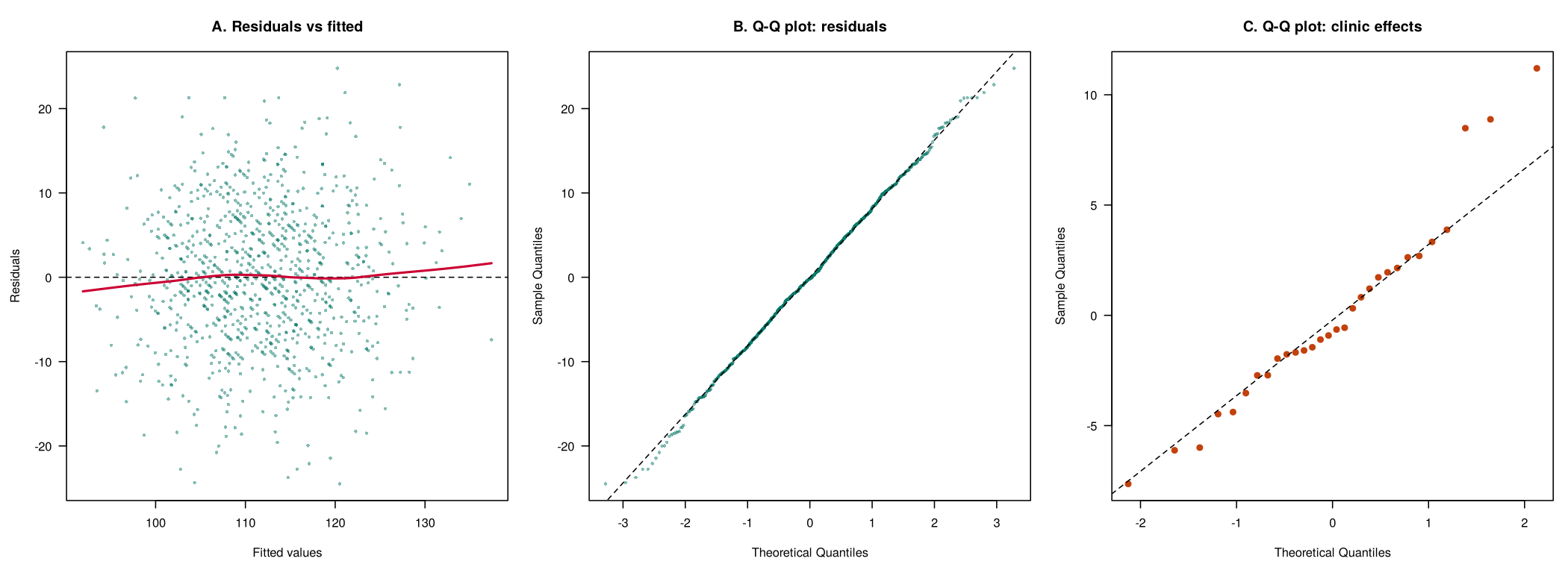
In this example the residual checks look acceptable, there are 30 clinics, and the model is not singular. With fewer than about 40 clusters, a small-sample correction to the tests is advised (Hemming & Taljaard, 2023), and the lmerTest output in this section already uses one (Satterthwaite's method). The three high clinics in panel C are a mild departure from normal cluster effects. Fixed-effect estimates are usually not very sensitive to this assumption, but the clinics themselves might be examined, for example to see whether they serve an older population or record blood pressure differently.

The checks support the random-intercept model for the clinic data. The final part of this section considers a more flexible model, in which the effect of a predictor may differ between clinics.

Random Slopes

The random-intercept model lets clinic baselines differ but assumes that each predictor has the same effect in every clinic. A random slope lets the effect of a predictor vary between clusters as well. In lmer(), a random slope for age is written (age | clinic_id), which gives each clinic its own intercept and its own age slope. Random slopes suit research questions about how an effect differs between settings, such as whether a program works better in some schools than others. They need more clusters and more observations per cluster, and with 30 clinics they often produce a singular fit or a convergence warning. This lesson fits random intercepts only.

This section has fitted a linear mixed model with a random intercept for each clinic, shown how to read its fixed effects, variance components and adjusted ICC, and checked it against the assumptions in Table 5.5. Activity 5.2 fits the same model in R and runs the checks, and the knowledge check that follows tests the main ideas of the section. Section 3 applies the same approach to a binary outcome.

library(lmerTest)   # loads lme4 and adds p-values to lmer() output
clinics <- read.csv("phaa_clinics.csv")   # file must be in the working directory
clinics$clinic_id <- factor(clinics$clinic_id)
clinics$smoker <- factor(clinics$smoker, levels = c("No", "Yes"))
clinics$clinic_urban <- factor(clinics$clinic_urban, levels = c("rural", "urban"))
lmm <- lmer(sbp ~ age + female + smoker + clinic_urban + (1 | clinic_id), data = clinics)
summary(lmm)

confint(lmm, parm = "beta_", method = "Wald")   # 95% CIs for the fixed effects
vc <- as.data.frame(VarCorr(lmm))
vc$vcov[1] / sum(vc$vcov)                        # ICC after adjusting for the predictors

par(mfrow = c(1, 3))
plot(fitted(lmm), resid(lmm), main = "Residuals vs fitted"); abline(h = 0, lty = 2)
qqnorm(resid(lmm), main = "Q-Q: residuals"); qqline(resid(lmm))
qqnorm(ranef(lmm)$clinic_id[, 1], main = "Q-Q: clinic effects"); qqline(ranef(lmm)$clinic_id[, 1])
par(mfrow = c(1, 1))
isSingular(lmm)        # FALSE means the clinic variance was estimated without problems

Lesson 5 · Section 3

Binary Outcomes: Mixed Models and GEE

Two ways to allow for clustering when the outcome is yes or no.

The outcome

Specialist referral in 30 clinics

246

of 966 patients referred

25%

overall referral rate

30

clinics, with different referral rates

Referral is binary, so each method is a version of logistic regression that allows for the clinics.

Approach 1

The GLMM: logistic regression with a random intercept

glmer(referred ~ age + smoker + clinic_urban + (1 | clinic_id), family = binomial, data = clinics)

What it estimates

The odds ratios compare two patients in the same clinic, or in two clinics with the same baseline, so they are clinic-specific (conditional) odds ratios.

Clinic variation

The clinic shifts on the log-odds scale have a variance of 0.30 (standard deviation 0.55).

Approach 2

GEE: a population-averaged model with corrected standard errors

geeglm(referred ~ age + smoker + clinic_urban, id = clinic_id, family = binomial, corstr = "exchangeable", data = clinics)

What it estimates

The odds ratios describe the population as a whole, so they are population-averaged (marginal) odds ratios.

Working correlation

An exchangeable structure assumes that any two patients in a clinic are equally correlated, and here the correlation is estimated at 0.04.

Comparing the models

Smoking barely changes; urban clinic does

Two questions

Clinic-specific or population-averaged?

GLMM (clinic-specific)

This compares patients in the same clinic, or in clinics with the same baseline. Its odds ratios are usually a little further from 1. It suits questions about individual clinics.

GEE (population-averaged)

This compares referral across the whole population, averaged over all clinics. It suits questions about policy for the population.

For a continuous outcome, as in Section 2, the two kinds of estimate coincide.

Assumptions and checks

What to check in a GLMM and in GEE

Check	GLMM: glmer()	GEE: geeglm()
Binary outcome and enough events	Yes (about 10 per predictor)	Yes
Enough clusters	About 20 to 30	About 30 to 40 or more
Cluster effects	Assumed normal (log-odds scale)	No assumption about their shape
Warnings	Read convergence warnings	Check the cluster id and sort the data

Choosing a method

GLMM or GEE?

Question	Points to
Is the question about individual clusters?	GLMM
Is the question about the whole population?	GEE
Are there fewer than about 30 clusters?	GLMM
Is the variation between clusters of interest?	GLMM
Is the outcome continuous?	Linear mixed model (Section 2)

Both methods agree here: urban clinics refer more patients.

Carry forward

What to take into the next section

• A GLMM adds a random intercept to a logistic regression, and GEE fits a population-averaged logistic regression with standard errors that allow for clustering.
• The GLMM gives clinic-specific odds ratios and GEE gives population-averaged odds ratios.
• Both methods widen the standard errors of cluster-level predictors, and GEE needs more clusters.

Introduction and Overview

This section extends logistic regression to clustered data. The outcome is referred, which records whether each of the 966 patients in phaa_clinics.csv was referred to a specialist (246 were, or 25.5%). The predictors are age, smoking and urban clinic. The section fits a generalized linear mixed model (GLMM) and a generalized estimating equations (GEE) model, compares them with an ordinary logistic regression, and explains when each approach is preferred.

Two Ways to Allow for Clustering

Logistic regression can allow for clustering in two ways, which correspond to the two families of methods introduced in Section 1 and listed in Table 5.3. A GLMM gives each clinic its own baseline log-odds, and GEE fits one model for the whole population and calculates standard errors that allow for the clustering. The two subsections below describe each approach in turn.

The Generalized Linear Mixed Model

A generalized linear mixed model (GLMM) adds random effects to a generalized linear model. For a binary outcome, it is a logistic regression in which each clinic has its own baseline log-odds, with the clinic shifts drawn from a normal distribution. It is fitted with glmer() from lme4, which takes the same family = binomial argument as glm(). Equation 5.4 writes the GLMM for referral in the clinic data.

Generalized Estimating Equations

Generalized estimating equations (GEE) fit a logistic regression without clinic effects. A working correlation describes how alike patients in the same clinic are assumed to be, and GEE uses it to weight the data. The standard errors are then calculated from the variation between clinics, which allows for the clustering (Zeger & Liang, 1986). The analyst chooses the working correlation structure. For people in clinics, schools or households, the usual choice is "exchangeable", which assumes that any two members of a cluster are equally correlated. The corrected (sandwich) standard errors remain valid even if the working correlation is not exactly right, provided there are enough clusters. GEE is fitted with geeglm() from geepack, which needs the cluster identifier in the id argument and the data sorted so that each cluster's rows are together.

The three flip cards below define terms that recur in the rest of this section: the clinic-specific odds ratio that a GLMM estimates, the population-averaged odds ratio that GEE estimates, and the working correlation that GEE uses.

The two approaches therefore estimate different quantities: the GLMM gives clinic-specific odds ratios and GEE gives population-averaged odds ratios. The next part fits both models to the referral data and compares their results with an ordinary logistic regression.

Comparing the Results

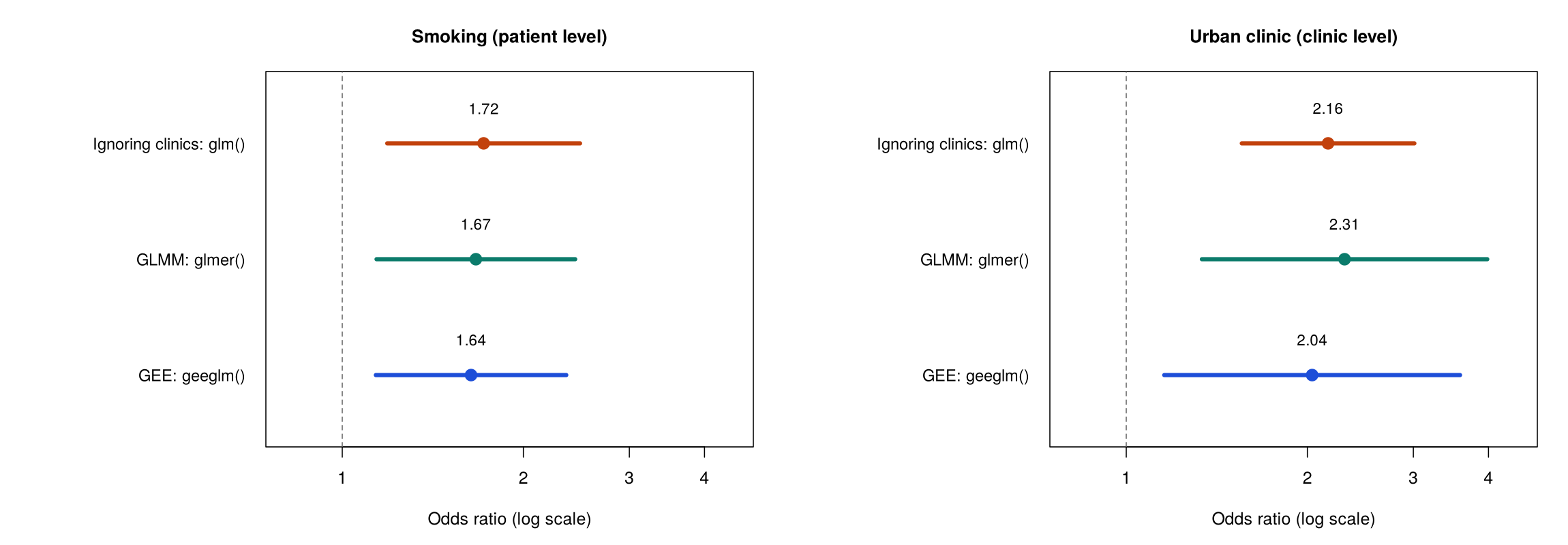
Activity 5.3 below fits an ordinary logistic regression (glm()), a GLMM (glmer()) and GEE (geeglm()) with the same three predictors. Table 5.6 shows the odds ratios for smoking (a patient-level predictor) and urban clinic (a clinic-level predictor), with their standard errors on the log-odds scale.

Table 5.6. Odds ratios for smoking and urban clinic, with standard errors on the log-odds scale, from three models of specialist referral.

Figure 5.6 plots the same odds ratios with their 95% confidence intervals.

For smoking, the three models give similar odds ratios and standard errors, because smokers and non-smokers are found in every clinic and the comparison can be made within clinics. For urban clinic, the standard error rises from 0.168 in the ordinary logistic regression to 0.279 in the GLMM and 0.289 in GEE, an increase of about 70%. The odds ratio remains clearly above 1 in all three models: patients in urban clinics have about twice the odds of referral of patients in rural clinics of the same age and smoking status (GLMM OR 2.31, p = 0.003; GEE OR 2.04, p = 0.014).

The GEE odds ratio for urban clinics (2.04) is a little lower than the glm() odds ratio (2.16) because the exchangeable working correlation gives each patient in a large clinic slightly less weight. Refitting GEE with corstr = "independence" reproduces the glm() odds ratio of 2.16, with the corrected standard error of 0.289.

Worked Example 5.3 explains why the GLMM odds ratio for urban clinics in Table 5.6 is further from 1 than the GEE odds ratio.

The GLMM and GEE agree that urban clinics have about twice the odds of referral, and the validity of each result rests on assumptions that the next part sets out.

Assumptions and How to Check Them

The GLMM and GEE share some assumptions and differ in others, including the number of clusters each needs. Table 5.7 lists the assumptions of each approach with how to check them, and Box 5.2 describes a step that GEE requires before the model is fitted.

Table 5.7. Assumptions of the logistic GLMM and GEE, with how to check them.

With 30 clinics, the referral data meet the GLMM requirement for the number of clusters and sit at the lower limit for GEE. The checks alone therefore leave the choice between the two models open, and the next part turns to the research question.

Choosing Between a GLMM and GEE

The choice depends mainly on the research question (Subramanian & O'Malley, 2010). A GLMM suits questions about individual clusters, estimates how much the clusters vary, and works with fewer clusters. GEE suits questions about the population as a whole, makes no assumption about the distribution of cluster effects, and needs more clusters for reliable standard errors (Hubbard et al., 2010). In practice, many epidemiological papers report one approach as the main analysis and the other as a sensitivity analysis. When they agree, as they do for urban clinics here, the conclusion is stronger.

This section has fitted a GLMM and GEE to a binary outcome and shown that both widen the standard error for the clinic-level predictor while reaching the same conclusion for urban clinics. Activity 5.3 fits the three models in Table 5.6 in R and compares them, and the knowledge check that follows tests the main ideas of the section. Section 4 applies a linear mixed model and GEE to repeated measurements of the same people.

library(lme4); library(geepack)   # glmer() for the GLMM, geeglm() for GEE
clinics <- read.csv("phaa_clinics.csv")   # file must be in the working directory
clinics$clinic_id <- factor(clinics$clinic_id)
clinics$smoker <- factor(clinics$smoker, levels = c("No", "Yes"))
clinics$clinic_urban <- factor(clinics$clinic_urban, levels = c("rural", "urban"))
table(clinics$referred)                  # 1 = referred to a specialist
naive <- glm(referred ~ age + smoker + clinic_urban, family = binomial, data = clinics)
glmm  <- glmer(referred ~ age + smoker + clinic_urban + (1 | clinic_id),
               family = binomial, data = clinics)
summary(glmm)

clinics <- clinics[order(clinics$clinic_id), ]   # GEE needs each clinic's rows together
gee <- geeglm(referred ~ age + smoker + clinic_urban, id = clinic_id,
              family = binomial, corstr = "exchangeable", data = clinics)
summary(gee)
options(digits = 7)   # summary() of a GEE model lowers the printed digits; this restores the default

# Odds ratios and standard errors for urban clinics from the three models
se <- function(fit) summary(fit)$coefficients["clinic_urbanurban", 2]
b  <- c(naive = coef(naive)[["clinic_urbanurban"]], glmm = fixef(glmm)[["clinic_urbanurban"]],
        gee = coef(gee)[["clinic_urbanurban"]])
round(cbind(OR = exp(b), SE = c(se(naive), se(glmm), se(gee))), 3)

Lesson 5 · Section 4

Repeated Measures Over Time

When the same people are measured several times, each person becomes a cluster of visits.

Running example

A wellness trial with four visits

200

adults, 100 per arm

4

visits: 0, 6, 12 and 18 months

2

outcomes: blood pressure and adherence

Each person is a cluster of visits, so the visits from one person are not independent.

Data layout

Long format: one row per visit

id	arm	visit (months)	sbp_mmhg	adherent
R0001	control	0	132	0
R0001	control	6	131	0
R0001	control	12	141	0
R0001	control	18	126	0
R0002	control	0	127	1

Mixed models and GEE need long format, with an id column that identifies the person (the cluster).

Look first

Individual lines and arm averages

Missed visits

Mixed models use every visit that was attended

96

of 800 measurements missing (12%)

121

of 200 people attended all four visits

704

measurements used by the mixed model

The results are valid if missing a visit depends only on information in the model (missing at random).

The model

Does blood pressure fall faster in the intervention arm?

lmer(sbp_mmhg ~ arm * visit + (1 | id), data = visits)

Term	What it measures
(1 | id)	A baseline level for each person (random intercept)
armintervention	The difference between the arms at the start (month 0)
visit	The change per month in the control arm
armintervention:visit	The extra change per month in the intervention arm

Reading the output

An extra fall of about 2.7 mmHg over 18 months

Term	Estimate	SE	p-value
Intervention arm at month 0	−1.32 mmHg	1.07	0.22
Change per month, control arm	−0.160 mmHg	0.043	< 0.001
Extra change per month, intervention arm	−0.149 mmHg	0.061	0.014

−2.7

mmHg extra over 18 months (18 × −0.149)

0.56

ICC: how alike each person's visits are

A repeated binary outcome

Adherence over time

Reading the output

Adherence rises faster in the intervention arm

Term	Odds ratio	95% CI
Intervention arm at month 0	1.00	0.60 to 1.69
Change per month, control arm	0.99	0.96 to 1.02
Extra change per month, intervention arm	1.093	1.041 to 1.147

Over one six-month interval, 1.093⁶ ≈ 1.7. The working correlation between a person's visits is 0.07, and there are 200 clusters.

Assumptions and checks

What to check in a repeated-measures analysis

Check	How
Long format with a person identifier	head(data); sort by id and visit for GEE
Time coded and shaped correctly	Plot the averages by visit; straight lines support a linear trend
Residuals for the mixed model	The residual and Q-Q plots from Section 2
Missed visits	Count them by visit and compare people who missed visits with those who did not

Lesson summary

Data structure, model and main check

Situation	Model and R function	Main check
Any clustered data	ICC and design effect	How strong is the clustering, and how much information is lost?
Continuous outcome	Linear mixed model, lmer()	Residual plots, Q-Q of cluster effects, number of clusters
Binary outcome, cluster-specific	GLMM, glmer()	Events, convergence warnings
Binary outcome, population-averaged	GEE, geeglm()	About 30 to 40 clusters or more, sorted data
Repeated measures	The same models with the person as the cluster	Long format, time trend, missed visits

Introduction and Overview

This section applies the methods of the lesson to repeated measures, in which the same people are measured at several times. The example is phaa_repeated.csv, a simulated wellness trial in which 200 adults were assigned to a control arm or an intervention arm (100 each) and were due to attend visits at 0, 6, 12 and 18 months. At each visit the study recorded systolic blood pressure (sbp_mmhg) and whether the person was adhering to the program (adherent = 1). The section covers the layout of repeated-measures data, missed visits, a linear mixed model for the change in blood pressure, and GEE for the repeated binary outcome.

Repeated Measures as Clustered Data

When the same person is measured more than once, the measurements share that person's genes, habits, circumstances and baseline health, so they are more alike than measurements from different people. Each person is therefore a cluster of visits, and the methods from the earlier sections apply with the person in place of the clinic. In this trial, the ICC for blood pressure is 0.56: more than half of the variation is a stable difference between people, much more than the clustering of patients in clinics.

The two subsections below describe how the trial data are laid out for these methods and what a plot of the data shows about the dependence.

Long and Wide Format

Repeated-measures data can be stored in wide format, with one row per person and a column for each visit, or in long format, with one row per visit and columns for the person identifier, the visit time and the outcome. Mixed models and GEE in R need long format. The trial file is already in long format, with 800 rows (200 people × 4 visits). Table 5.8 shows the first five rows of the file.

Table 5.8. The first five rows of phaa_repeated.csv in long format, with one row per visit.

The id column identifies the person (the cluster), visit records months since the start, and each person appears once for each visit. In wide format, the same person R0001 would be a single row with columns such as sbp_0, sbp_6, sbp_12 and sbp_18. The base R function reshape() or tidyr::pivot_longer() converts wide data to long format.

Looking at the Data

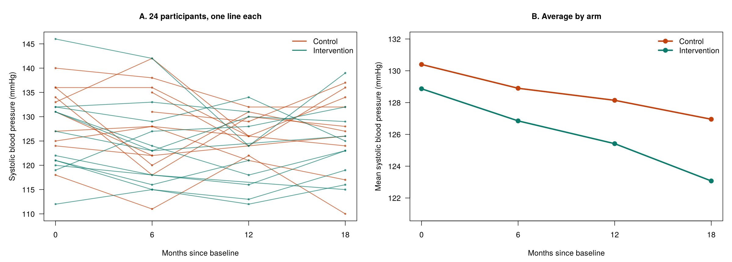
Before any model is fitted, a plot of the measurements over time shows how strongly each person’s visits are linked and what shape the trend takes. Figure 5.7 shows the blood pressure of individual participants at each visit and the average in each arm.

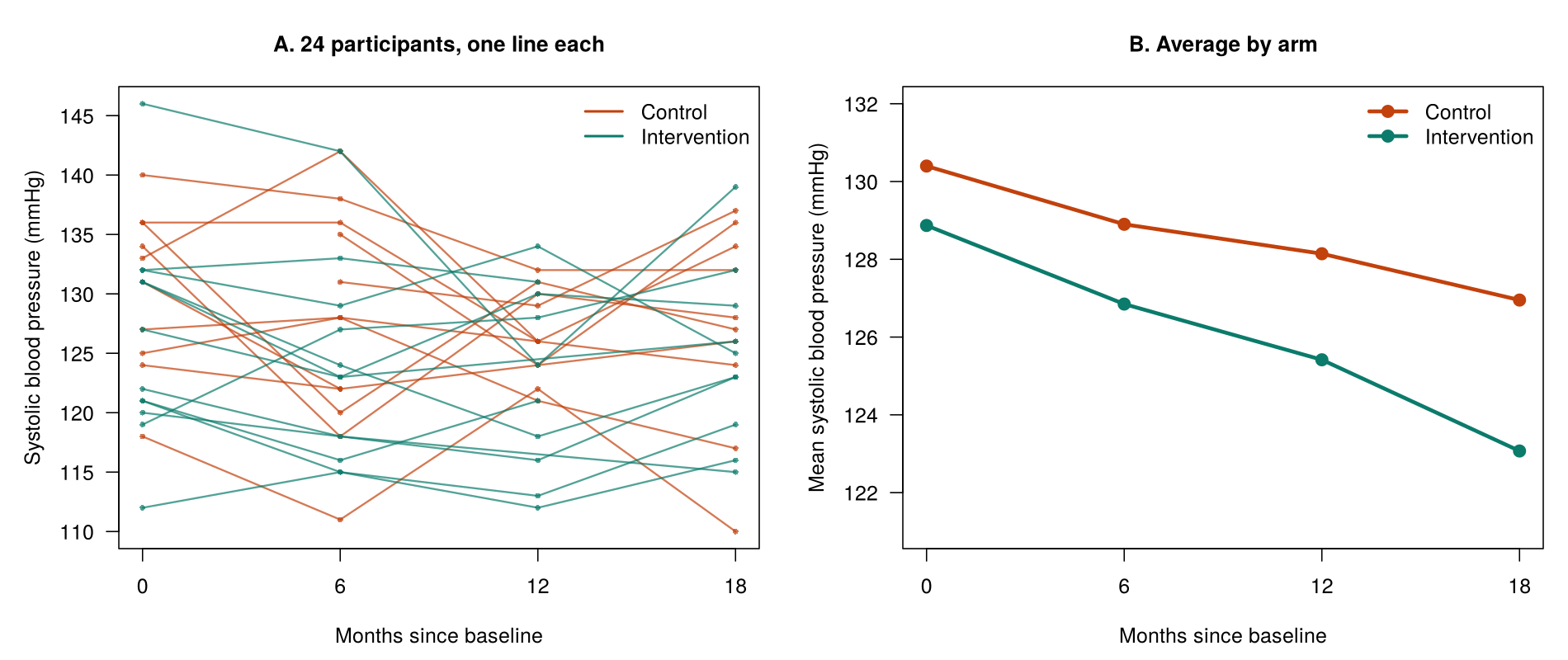
The spaghetti plot (panel A) shows the dependence directly: people start at very different levels and tend to stay there. The averages (panel B) fall in both arms, from 130.4 to 127.0 mmHg in the control arm and from 128.9 to 123.1 mmHg in the intervention arm, and the roughly straight lines suggest that a linear trend over time is reasonable.

The trial data are therefore in the long format that the models need, and Figure 5.7 shows both the dependence within people and a roughly linear trend. Some planned visits were missed, however, and the next part considers how missed visits affect the analysis.

Missed Visits

Of the 800 planned measurements of blood pressure, 96 (12%) are missing, and only 121 of the 200 participants attended all four visits. Dropping everyone with a missed visit (a complete-case analysis) would discard 79 people and could bias the results if the people who missed visits differ from those who attended every one. For a regression model, a complete-case analysis still gives unbiased coefficients when the chance that a record is incomplete depends only on the predictors in the model and not on the outcome, although it loses precision; this exception refines the statement in Lesson 2 that listwise deletion is biased unless the data are MCAR. In repeated-measures data a missed visit often depends on the person’s earlier outcome values, and then the exception does not apply. A mixed model uses every measurement that was taken, here 704 measurements from all 200 people.

Box 5.3 recalls the three missing-data mechanisms from Lesson 2 and ends with a retrieval question, and Box 5.4 restates the missing-at-random condition in plain terms for the trial.

When the missing-at-random condition holds, a mixed model fitted to all 704 available measurements gives valid results. The next part fits that model to the blood pressure data.

A Mixed Model for Change Over Time

The model for blood pressure includes a random intercept for each person and fixed effects for arm, visit and their interaction. Equation 5.5 writes the model.

Table 5.9 gives the estimates of the fixed effects for arm, visit and their interaction, with an interpretation of each.

Table 5.9. Fixed effects from the random-intercept model for blood pressure over time.

Over the 18 months of the trial, the extra fall in the intervention arm is 18 × −0.149 = −2.7 mmHg. The random effects give a between-person variance of 34.80 and a within-person variance of 27.58, so the ICC is 34.80 ÷ (34.80 + 27.58) = 0.56.

Worked Example 5.4 combines the intercept of the model with the estimates in Table 5.9 to predict blood pressure at month 18 in each arm.

The accordion below describes two extensions of this model, random slopes for time and a correlation that depends on the time between visits, both of which are beyond the scope of this lesson.

The mixed model shows an extra fall of about 2.7 mmHg over 18 months in the intervention arm. The trial also recorded a binary outcome at each visit, and the next part models it with GEE.

GEE for a Repeated Binary Outcome

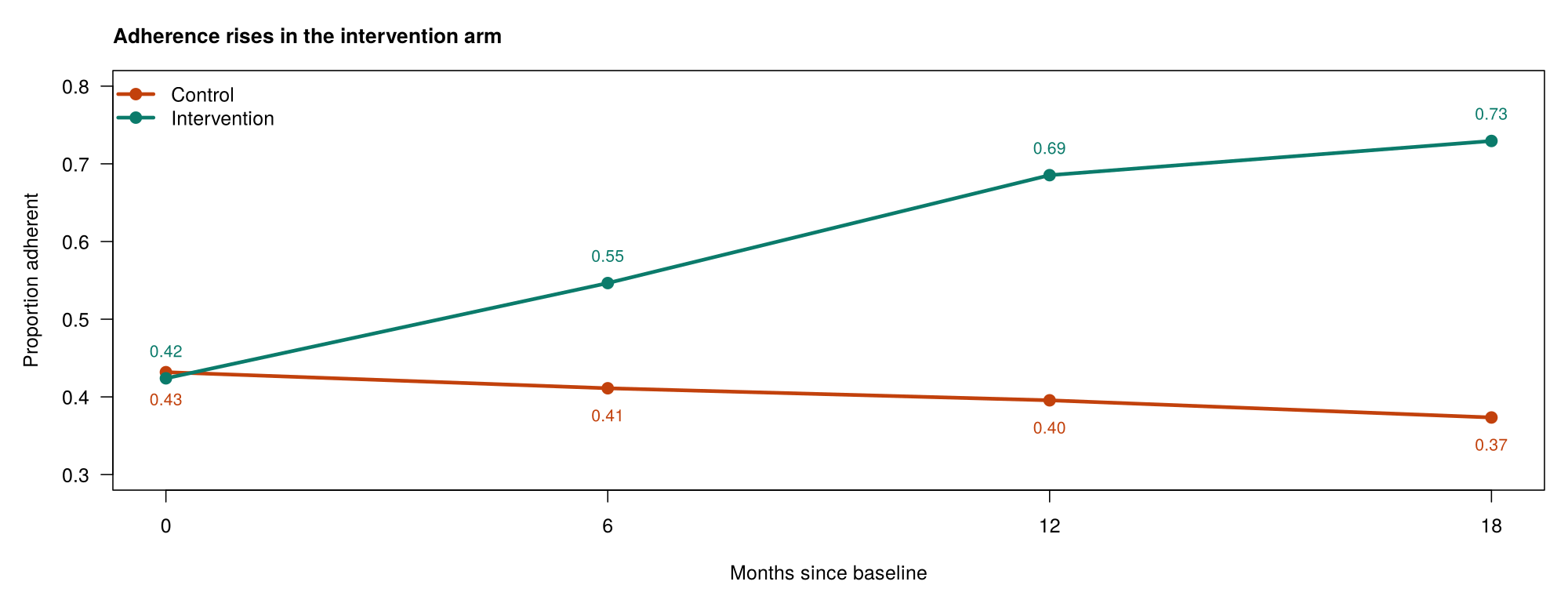
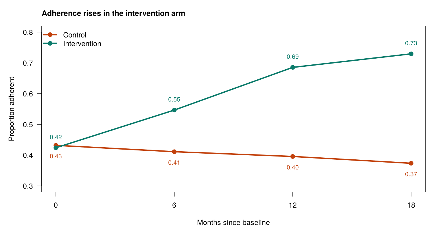
Adherence is recorded as yes or no at each visit. The share adherent falls slightly in the control arm (0.43 at month 0 to 0.37 at month 18) and rises steadily in the intervention arm (0.42 to 0.73). Figure 5.8 shows these proportions at each visit.

A GEE model with the person as the cluster gives population-averaged odds ratios for the trial, which matches the question of how the program changes adherence across participants. With 200 people there are plenty of clusters for the corrected standard errors. Table 5.10 gives the odds ratios from this model.

Table 5.10. Odds ratios from the GEE model for adherence over time.

Over one six-month interval between visits, the interaction corresponds to an odds ratio of 1.093⁶ ≈ 1.70. The estimated exchangeable correlation between a person's visits is 0.07, much weaker than the correlation for blood pressure, but GEE allows for it in the standard errors.

GEE needs a stronger condition about missed visits than the mixed model. Its results are valid when the chance of missing a visit depends only on the predictors in the GEE model, here arm and visit. If missed visits depend on earlier outcomes, such as earlier blood pressure or adherence, a mixed model, or a weighted form of GEE that is beyond this lesson, is preferred.

GEE therefore shows a steady rise in adherence in the intervention arm, provided that missed visits depend only on arm and visit. The next part collects the checks that apply to both repeated-measures models.

Assumptions and How to Check Them

A repeated-measures analysis needs some of the checks from the earlier sections together with checks of its own, which concern the layout of the data, the coding of time and the missed visits. Table 5.11 lists them for the mixed model and for GEE.

Table 5.11. Assumptions and requirements of a repeated-measures analysis, with how to check them.

These checks complete the analysis of the wellness trial. The final part sets the four examples of the lesson side by side.

Bringing the Lesson Together

The four sections of this lesson apply one approach. The cluster variable is identified first, the clustering is measured with the ICC, and a model is chosen that allows for it: a linear mixed model for a continuous outcome, a GLMM or GEE for a binary outcome, and the same models with the person as the cluster for repeated measures. Table 5.12 summarises the four examples with the cluster, the model and R function, and the main result of each.

Table 5.12. The four examples of the lesson, with the cluster, model and main result of each.

Activity 5.4 fits the mixed model for blood pressure over time in R, and Activity 5.5 continues from it with the GEE model for adherence. The knowledge check that follows the two activities tests the main ideas of this section, and the final page of the lesson gathers the key takeaways and the final assessment.

library(lmerTest)   # loads lme4 and adds p-values
visits <- read.csv("phaa_repeated.csv")   # file must be in the working directory
visits$id  <- factor(visits$id)
visits$arm <- factor(visits$arm, levels = c("control", "intervention"))
head(visits, 8)                                      # long format: one row per visit
table(visit = visits$visit, missing = is.na(visits$sbp_mmhg))
round(tapply(visits$sbp_mmhg, list(visits$arm, visits$visit), mean, na.rm = TRUE), 1)

lmm_t <- lmer(sbp_mmhg ~ arm * visit + (1 | id), data = visits)
summary(lmm_t)

vc <- as.data.frame(VarCorr(lmm_t))
vc$vcov[1] / sum(vc$vcov)                            # how alike one person's visits are
18 * fixef(lmm_t)[["armintervention:visit"]]          # extra change over 18 months

library(geepack)
adh <- visits[!is.na(visits$adherent), ]             # visits with adherence recorded
adh <- adh[order(adh$id, adh$visit), ]               # each person's rows together
round(tapply(adh$adherent, list(adh$arm, adh$visit), mean), 2)   # share adherent
gee_a <- geeglm(adherent ~ arm * visit, id = id, family = binomial,
                corstr = "exchangeable", data = adh)
summary(gee_a)
options(digits = 7)   # restore the default number of printed digits

round(exp(cbind(OR = coef(gee_a), confint.default(gee_a))), 3)   # odds ratios, 95% CIs

Bringing It All Together

This lesson addressed the assumption of independence that every model in the previous lessons shares. Section 1 showed that observations are dependent when they share a cluster, such as patients in the same clinic or visits by the same person. The intracluster correlation coefficient measured the clustering in the clinic data (0.175 for systolic blood pressure), the design effect of 6.45 showed that the 966 patients carried about as much information as 150 independent patients, and an ordinary regression that ignored the clinics gave a standard error for urban clinics of 0.74 mmHg, compared with 1.96 mmHg from a model that allowed for them.

Section 2 fitted a linear mixed model with a random intercept for each clinic using lmer(). Its fixed effects were read like the coefficients of a linear regression, its random effects gave a clinic variance and a residual variance whose ratio was the adjusted ICC of 0.24, and it was checked with residual plots, a Q-Q plot of the clinic effects, the number of clinics and a test for a singular fit. Section 3 turned to a binary outcome, specialist referral, and compared a logistic mixed model fitted with glmer(), which gives cluster-specific odds ratios, with GEE fitted with geeglm(), which gives population-averaged odds ratios with sandwich standard errors. Section 4 treated each person in a wellness trial as a cluster of visits, arranged the data in long format, and used a mixed model for blood pressure and GEE for adherence, each with an arm-by-visit interaction that answered the main question of the trial and each using every visit that was attended.

Across the lesson, the same steps were followed each time: the cluster variable was identified, the clustering was measured, a model that allows for it was chosen to suit the outcome type and the research question, and the model's assumptions were checked before the results were reported. The final assessment asks for these steps to be applied to new studies.

The final assessment covers all four sections. All 15 questions must be answered correctly (100%), and the final reflection completed, to finish the lesson.

Final Knowledge Assessment